spa (System Identification Toolbox)

Estimate frequency response and spectrum by spectral analysis.

Syntax

g = spa(data)
g = spa(data,M,w,maxsize)
[g,phi,spe] = spa(data)

Description

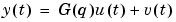
spa estimates the transfer function g and the noise spectrum of the general linear model

where is the spectrum of .

data contains the output-input data as an iddata object. The data may be complex-valued.

g is returned as an idfrd object (see idfrd) with the estimate of at the frequencies specified by row vector w. The default value of w is

```
w = [1:128]/128*pi/Ts
```

Here Ts is the sampling interval of data.

g also includes information about the spectrum estimate of at the same frequencies. Both outputs are returned with estimated covariances, included in g. See idfrd.

M is the length of the lag window used in the calculations. The default value is

```
M = min(30,length(data)/10)
```

Changing the value of M exchanges bias for variance in the spectral estimate. As M is increased, the estimated functions show more detail, but are more corrupted by noise. The sharper peaks a true frequency function has, the higher M it needs. See etfe as an alternative for narrowband signals and systems. See also Estimating Spectra and Frequency Functions in the "Tutorial".

maxsize controls the memory-speed trade-off (see Algorithm Properties).

For time series, where data contains no input channels, g is returned with the estimated output spectrum and its estimated standard deviation.

When spa is called with two or three output arguments:

g is returned as an idfrd model with just the estimated frequency response from input to output and its uncertainty.
phi is returned as an idfrd model, containing just the spectrum data for the output spectrum and its uncertainty.
spe is returned as an idfrd model containing spectrum data for all output-input channels in data. That is if z = [data.OutputData, data.InputData], spe contains as spectrum data the matrix-valued power spectrum of z.

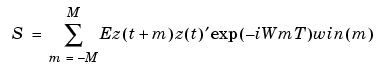
Here win(m) is weight at lag m of an M-size Hamming window and W is the frequency value i rad/s. Note that ' denotes complex-conjugate transpose.

The normalization of the spectrum differs from the one used by spectrum in the Signal Processing Toolbox. See Spectrum Normalization and the Sampling Interval in the "Tutorial" for a more precise definition.

Examples

With default frequencies

```
g = spa(z);
bode(g)
```

With logarithmically spaced frequencies

w = logspace(-2,pi,128);
g= spa(z,[],w); % (empty matrix gives default)
bode(g,3)
bode(g('noise'),3) % The noise spectrum with confidence interval 
of 3 standard deviations.

Algorithm

The covariance function estimates are computed using covf. These are multiplied by a Hamming window of lag size M and then Fourier transformed. The relevant ratios and differences are then formed. For the default frequencies, this is done using FFT, which is more efficient than for user-defined frequencies. For multi-variable systems, a straightforward for-loop is used.

Note that M = is in Table 6.1 of Ljung (1999). The standard deviations are computed as on pages 184 and 188 in Ljung (1999).

size ss, tf, zpk, frd