idss (System Identification Toolbox)

Package state-space parameterizations into an idss model.

Syntax

m = idss(A,B,C,D)
m = 
idss(A,B,C,D,K,x0,Ts,'Property1',Value1,...,'PropertyN',ValueN)
mss = idss(m1)

Description

The function idss is used to construct state-space model structures with various parameterizations. It is a complement to idgrey and deals with parameterizations that do not require the user to write a special M-file. Instead it covers parameterizations that either a completely 'Free', that is, all parameters in the A, B and C matrices can be adjusted freely, or 'Canonical', meaning that the matrices are parameterized as canonical forms. The parameterization can also be 'Structured', which means that certain elements in the state-space matrices are free to be adjusted, while other are fixed. This is explained below.

Ts is the sampling interval. Ts = 0 means a continuous time model.

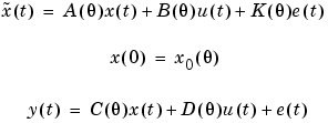
The idss object m describes state-space models in innovations form, of the following kind.

Here is the time derivative for a continuous time model and for a discrete time model.

The model m will contain information both about the nominal/initial values of the A, B, C, D, K, and X0-matrices and about how these matrices are parameterized by the parameter vector (to be estimated).

The nominal model is defined by idss(A,B,C,D,K,X0). If K and X0 are omitted they are taken as zero matrices of appropriate dimensions.

Defining an idss object from a given model

```
mss = idss(m1)
```

constructs an idss model from any idmodel or LTI-system m1.

If m1 is an LTI system (ss, tf or zpk) which has no InputGroup called 'Noise', the corresponding state-space matrices A,B,C,D are used to define the idss object. The Kalman gain K is then set to zero.

If the LTI-system has an InputGroup called 'Noise', these inputs will be interpreted as white noise with a covariance matrix equal to the identity matrix. The corresponding Kalman gain and noise variance is then computed and entered into the idss model together with A,B,C, and D.

Parameterizations

There are several different ways to define the parameterization of the state-space matrices. The parameterization will determine which parameters can be adjusted to data by the parameter estimation routine pem:

Free Black-Box parameterizations: This is the default situation and corresponds to letting all parameters in A, B, and C be freely adjustable. This is obtained by setting the property 'SSParameterization' = 'Free'. The parameterizations of D, K, and X0 are then determined by the following properties:

'nk': A row vector of the same length as the number of inputs. The ku-th element is the delay from input channel no ku. nk =[0,...,0], thus means that there is no delay from any of the inputs, and that consequently all elements of the D matrix should be estimated. nk =[1,...,1] means that there is a delay of 1 from each input, so that the D matrix is fixed to be zero.
'DisturbanceModel': This property affects the parametrization of K and can assume the values:

'Estimate' which means that all elements of the K matrix are to be estimated.
'None': all elements of K are fixed to zero.
'Fixed': all elements of K are fixed to their nominal/initial values.

'InitialState': This properly affects the parameterization of X0 and can assume the following values:

'Auto': An automatic choice of the below is made, depending on data (default).
'Estimate': All elements of X0 are to be estimated.
'Zero': All elements of X0 are fixed to zero.
'Fixed': All elements of X0 are fixed to their nominal/initial values.
'Backcast': The vector X0 is adjusted, during the parameter estimation step, to a suitable value, but it is not stored as an estimation result.

Canonical Black-Box parameterizations: This is obtained by setting the property 'SSParameterization' = 'Canonical'. The matrices A, B and C are then parameterized as an observer canonical form, which means that ny (= the number of output channels) rows of A are fully parameterized while the others contain 0's and 1's in a certain pattern. The C matrix is built up of 0's and 1's while the B matrix is fully parameterized. See Equation(A.16) in Ljung(1999) for details. The exact form of the parameterization is affected by the property 'CanonicalIndices'. The default value 'Auto' is a good choice. The parameterization of the D, K and X0-matrices in this case is determined by the properties 'nk', 'DisturbanceModel' and 'InitialState' exactly as above.
Arbitrarily structured parameterizations: To cover the general case where arbitrary elements of the state-space matrices may be fixed and others be freely adjusted, corresponds to the case 'SSParameterization' = 'Structured'. Then the parameterization is determined by the idss properties As, Bs, Cs, Ds, Ks, and X0s. These are the structure matrices that are "shadows" of the state-space matrices, so that an element in these matrices that is equal to NaN indicates a freely adjustable parameter, while a numerical value in these matrices indicates that the corresponding system matrix element is fixed (nonadjustable) to this value.

See the Examples below.

idss Properties

To summarize the properties of the idss object we have:

SSParameterization with possible values

'Free': Means that all parameters in A,B and C are freely adjustable and the parameterizations of D, K and X0 depend on the properties 'nk', 'DisturbanceModel' and 'InitialState'
'Canonical': Means that A and C are parameterized as an observer canonical form. The details of this parameterization depends on the property 'CanonicalIndices'. The B-matrix is always fully parameterized, and the parameterizations of D, K, and X0 depend on the properties 'nk', 'DisturbanceModel', and 'InitialState'.
'Structured': Means that the parametrization is determined by the properties (the structure matrices) 'As', 'Bs', 'Cs', 'Ds', 'Ks', and 'X0s'. A NaN in any position in these matrices denotes a freely adjustable parameter and a numeric value denotes a fixed and nonadjustable parameter.
nk: A row vector with as many entries as the number of input channels. The entry number k denotes the time delay from input number k to y(t). This property is relevant only for 'Free' and 'Canonical' parameterizations. If any delay is larger than 1, the structure of the A, B, and C matrices will accommodate this delay, at the price of a higher order model.

DisturbanceModel with possible values:

'Estimate': Means that the K matrix is fully parameterized.
'None': Means that the K matrix is fixed to zero. This gives a so-called Output-Error model, since the model output depends on past inputs only.
'Fixed': Means that the K matrix is fixed to the current nominal values

InitialState with possible values:

'Estimate': Means that X0 is fully parameterized.
'Zero': Means that X0 is fixed to zero.
'Fixed': Means that X0 is fixed to the current nominal value.
'Backcast': The value of X0 is estimated by the identification routines as the best fit to data, but it is not stored.
'Auto': Gives an automatic, and data-dependent choice between 'Estimate', 'Zero' and 'Backcast'.

A, B, C, D, K, and X0: The state-space matrices that can be set and retrieved at any time. These contain both fixed values and estimated/nominal values.
dA, dB, dC, dD, dK, and dX0: The estimated standard deviations of the state-space matrices. These cannot be set, only retrieved. Note that these are not defined for an idss model with 'Free' SSParameterization. You can then convert the parameterization to 'Canonical' and study the uncertainties of the matrix elements in that form.
As, Bs, Cs, Ds, Ks, and X0s: These are the structure matrices that have the same sizes as A, B, C etc. and show the freely adjustable parameters as NaN in the corresponding position. These properties are used to define the model structure for 'SSParameterization' = 'Structured'. They are however always defined and can be studied also for the other parametrizations.
CanonicalIndices: Determines the details of the canonical parameterization. It is a row vector of integers with as many entries as there are outputs. They sum up to the system order. This is the so-called pseudo-canonical multi-index, with an exact definition, e.g., on page 132 in Ljung (1999). A good default choice is 'Auto'. This property is relevant only for the canonical parameterization case. Note however, that for 'Free' parameterizations, the estimation algorithms also store a canonically parameterized model, to handle the model uncertainty.

In addition to these properties, idss objects also have all the properties of the idmodel object. See idmodel properties, Algorithm Properties, and EstimationInfo.

Note that all properties can be set and retrieved either by set/get or by subscripts. Autofill applies to all properties and values, and are case insensitive.

m.ss='can'
set(m,'ini','z')
p = eig(m.a)

For a complete list of property values, use get(m). To see possible value assignments, use set(m). See also idprops idss.

Examples

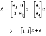
Define a continuous-time model structure corresponding to

with initial values

and estimate the free parameters

A = [-0.2, 0; 0, -0.3]; B = [2;4]; C=[1, 1]; D = 0
m0 = idss(A,B,C,D);
m0.As = [NaN,0;0,NaN];
m0.Bs = [NaN;NaN];
m0.Cs = [1,1];
m0.Ts = 0;
m = pem(z,m0);

Estimate a model in free parameterization. Convert it to continuous time, then convert it to canonical form and continue to fit this model to data.

m1 = n4sid(data,3);
m1 = d2c(m1);
m1.ss ='can';
m = pem(data,m1);

All of this can be done at once by

```
m = pem(data,3,'ss','can','ts',0)
```

See Also

n4sid, pem

idpoly impulse