

| System Identification Toolbox | |
Estimate state-space models using a subspace method.
Syntax
Description
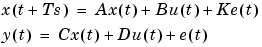
The function n4sid estimates models in state-space form, and returns them as an idss object m. It handles an arbitrary number of input and outputs, including the time-series case (no input). The state-space model is in the innovations form
m: The resulting model as an idss object.
data: An iddata object containing the output-input data.
order: The desired order of the state-space model. If order is entered as a row vector (like order = [1:10]), preliminary calculations for all the indicated orders are carried out. A plot will then be given that shows the relative importance of the dimension of the state vector. More precisely, the singular values of the Hankel matrices of the impulse response for different orders are graphed. You will be prompted to select the order, based on this plot. The idea is to choose an order such that the singular values for higher orders are comparatively small. If order = 'best', a model of "best" (default choice) order is computed, among the orders 1:10. This is the default choice of order.
The list of property name/property value pairs may contain any idss and algorithm properties. See idss and Algorithm Properties.
idss properties that are of particular interest for n4sid are:
nk: The delays from the inputs to the outputs, a row vector with the same number of entries as the number of input channels. Default is nk = [1 1 ... 1]. Note that delays being 0 or 1 show up as zeros or estimated parameters in the D matrix. Delays larger than 1 means that a special structure of the A, B and C matrices are used to accommodate the delays. This also means that the actual order of the state-space model will be larger than order.
CovarianceMatrix (can be abbreviated to 'co'): Setting CovarianceMatrix to 'None' will block all calculations of uncertainty measures. These may take the major part of the computation time. Note that, for a 'Free' parameterization, the individual matrix elements cannot be associated with any variance (these parameters are not identifiable). Instead, the resulting model m stores a hidden state-space model in canonical form, that contains covariance information. This is used when the uncertainty of various input-output properties are calculated. It can also be retrieved by m.ss = 'can'. The actual covariance properties of n4sid estimates are not known today. Instead the Cramer-Rao bound is computed and stored as an indication of the uncertainty.
DisturbanceModel: Setting DisturbanceModel to `None' will deliver a model with K = 0. This will have no direct effect on the dynamics model, other that that the default choice of N4Horizon will not involve past outputs.
InitialState: The initial state is always estimated for better accuracy. However. it is returned with m only if InitialState = `Estimate'.
Algorithm properties that are special interest are:
Focus: Assumes the values 'Prediction' (default), 'Simulation', ` Stability', or any SISO linear filter (given as an LTI or idmodel object, or as filter coefficients. See Algorithm Properties.) Setting 'Focus' to 'Simulation' chooses weights that should give a better simulation performance for the model. In particular, a stable model is guaranteed. Selecting a linear filter will focus the fit to the frequency ranges that are emphasized by this filter.
N4Weight: This property determines some weighting matrices used in the singular-value decomposition that is a central step in the algorithm. Two choices are offered: 'MOESP' that corresponds to the MOESP algorithm by Verhaegen, and 'CVA' which is the canonical variable algorithm by Larimore. The default value is 'N4Weight' = 'Auto', which gives an automatic choice between the two options. m.EstimationInfo.N4Weight tells you what the actual choice turned out to be.
N4Horizon: Determines the prediction horizons forward and backward, used by the algorithm. This is a row vector with three elements: N4Horizon =[r sy su], where r is the maximum forward prediction horizon, i.e., the algorithms uses up to r-step ahead predictors. sy is the number of past outputs, and su is the number of past inputs that are used for the predictions. See pages 209-210 in Ljung(1999) for the exact meaning of this. These numbers may have a substantial influence of the quality of the resulting model, and there are no simple rules for choosing them. Making 'N4Horizon' a k-by-3 matrix, means that each row of 'N4Horizon' will be tried out, and the value that gives the best (prediction) fit to data will be selected. (This option cannot be combined with selection of model order.) If the property 'Trace' is 'On', information about the results will be given in the MATLAB command window.
'N4Horizon', the interpretation is r=sy=su. The default choice is 'N4Horizon' = 'Auto', which uses an Akaike Information Criterion (AIC) for the selection of sy and su. If 'DisturbanceModel' = 'None', sy is set to 0. Typing m.EstimationInfor.N4Horizon will tell you what the final choice of horizons were.
Algorithm
The variants of the implemented algorithm are described in Section 10.6 in Ljung (1999).
Examples
Build a fifth order model from data with three inputs and two outputs. Try several choices of auxiliary orders. Look at the frequency response of the model.
Estimate a continuous-time model, in a canonical form parameterization, focusing on the simulation behavior. Determine the order yourself after seeing the plot of singular values.
See Also
idss, pem, Algorithm Properties
References
P. vanOverschee and B. DeMoor: Subspace Identification of Linear Systems: Theory, Implementation, Applications. Kluwer Academic Publishers, 1996.
M. Verhaegen: Identification of the deterministic part of MIMO state space models. Automatica, Vol 30, pp 61-74, 1994.
W.E. Larimore: Canonical variate analysis in identification, filtering and adaptive control. In Proc. 29th IEEE Conference on Decision and Control, pp 596-604, Honolulu, 1990.
| | nyquist | oe | |