
| Getting Started |   |
Linear-Quadratic-Gaussian (LQG) Design
Linear-quadratic-Gaussian (LQG) control is a modern state-space technique for designing optimal dynamic regulators. It enables you to trade off regulation performance and control effort, and to take into account process disturbances and measurement noise. Like pole placement, LQG design requires a state-space model of the plant (use ss to convert other model formats to state space). This section focuses on the continuous-time case (see the reference pages for dlqr and kalman for details on discrete-time LQG design).
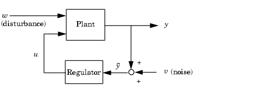
LQG design addresses the following regulation problem.

The goal is to regulate the output  around zero. The plant is subject to disturbances
  and is driven by controls
  . The regulator relies on the noisy measurements
  to generate these controls. The plant state and measurement equations are of the form
and both  and
and  are modeled as white noise.
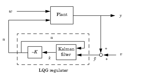
The LQG regulator consists of an optimal state-feedback gain and a Kalman state estimator. You can design these two components independently as shown next.
Optimal State-Feedback Gain
In LQG control, the regulation performance is measured by a quadratic performance criterion of the form

The weighting matrices Q, N, and R are user specified and define the trade-off between regulation performance (how fast  goes to zero) and control effort.
The first design step seeks a state-feedback law  that minimizes the cost function
  . The minimizing gain matrix
  is obtained by solving an algebraic Riccati equation. This gain is called the LQ-optimal gain.
Syntax. Given the (A,B,C,D) matrices of the system, and the weighting matrices Q, R, and N, use the lqr command to construct the LQ-optimal gain, K.
If N is omitted, by default its value is 0.
Kalman State Estimator
As in the case of pole placement, the LQ-optimal state feedback  is not implementable without full state measurement. It is possible, however, to derive a state estimate
  such that
  remains optimal for the output-feedback problem. This state estimate is generated by the Kalman filter

with inputs  (controls) and
  (measurements). The noise covariance data

determines the Kalman gain  through an algebraic Riccati equation.
The Kalman filter is an optimal estimator when dealing with Gaussian white noise. Specifically, it minimizes the asymptotic covariance

Syntax. Use the kalman function to construct a Kalman filter.
returns a state-space model kest of the Kalman estimator given the plant model sys_kf and the noise covariance data, Qn, Rn, and Nn. The plant model equations are the following.
where w and v are modeled as white noise. L is the Kalman gain and P the covariance matrix.
The figure below shows the required dimensions for Qn, Rn, and Nn. If Nn is 0, you can omit it
 .
.
Figure 4-50: Required Dimensions for Qn, Rn, and Nn
For a complete example of a Kalman filter implementation, see Kalman Filtering under "Design Case Studies" in the Control System Toolbox online documentation.
LQG Regulator
To form the LQG regulator, simply connect the Kalman filter and LQ-optimal gain  as shown below.

This regulator has state-space equations

Syntax. Assuming you have constructed the Kalman filter, kest, and the compensator, K, use the lqgreg command to create the LQG regulator.
See the example LQG Regulation under Design Case Studies online for a more complete discussion of construction LQG regulators.
LQG Design Tools
The Control System Toolbox contains functions to perform the three LQG design steps outlined above. These functions cover both continuous and discrete problems as well as the design of discrete LQG regulators for continuous plants. The following table summarizes the LQG design commands.
| Command |
Description |
|
Solve continuous-time algebraic Riccati equations |
|
Solve discrete-time algebraic Riccati equations |
|
LQ-optimal gain for discrete systems |
|
Kalman estimator |
|
Discrete Kalman estimator for continuous plant |
|
Form LQG regulator given LQ gain and Kalman filter |
|
LQ-optimal gain for continuous systems |
|
Discrete LQ gain for continuous plant |
|
LQ-optimal gain with output weighting |
 | Pole Placement | Example: LQG Design |  |