Optimization Toolbox

Quasi-Newton Methods

Of the methods that use gradient information, the most favored are the quasi-Newton methods. These methods build up curvature information at each iteration to formulate a quadratic model problem of the form

(3-3)

where the Hessian matrix, H, is a positive definite symmetric matrix, c is a constant vector, and b is a constant. The optimal solution for this problem occurs when the partial derivatives of x go to zero, i.e.,

(3-4)

The optimal solution point, , can be written as

(3-5)

Newton-type methods (as opposed to quasi-Newton methods) calculate H directly and proceed in a direction of descent to locate the minimum after a number of iterations. Calculating H numerically involves a large amount of computation. Quasi-Newton methods avoid this by using the observed behavior of f(x) and to build up curvature information to make an approximation to H using an appropriate updating technique.

A large number of Hessian updating methods have been developed. However, the formula of Broyden [3], Fletcher [14], Goldfarb [22], and Shanno [39] (BFGS) is thought to be the most effective for use in a General Purpose method.

The formula given by BFGS is

(3-6)

where

As a starting point, can be set to any symmetric positive definite matrix, for example, the identity matrix I. To avoid the inversion of the Hessian H, you can derive an updating method that avoids the direct inversion of H by using a formula that makes an approximation of the inverse Hessian at each update. A well known procedure is the DFP formula of Davidon [9], Fletcher, and Powell [16]. This uses the same formula as the BFGS method (Eq. 3-6) except that is substituted for .

The gradient information is either supplied through analytically calculated gradients, or derived by partial derivatives using a numerical differentiation method via finite differences. This involves perturbing each of the design variables, x, in turn and calculating the rate of change in the objective function.

At each major iteration, k, a line search is performed in the direction

(3-7)

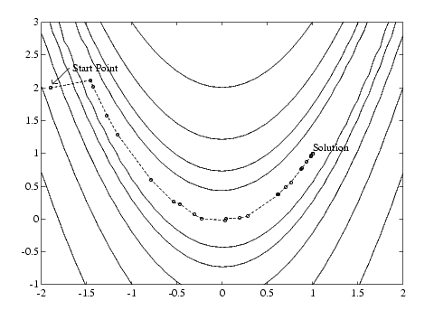
The quasi-Newton method is illustrated by the solution path on Rosenbrock's function (Eq. 3-2) in Figure 3-2, BFGS Method on Rosenbrock's Function. The method is able to follow the shape of the valley and converges to the minimum after 140 function evaluations using only finite difference gradients.

Figure 3-2: BFGS Method on Rosenbrock's Function

Unconstrained Optimization

Line Search