fseminf (Optimization Toolbox)

Find a minimum of a semi-infinitely constrained multivariable nonlinear function

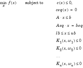
where x, b, beq, lb, and ub are vectors, A and Aeq are matrices, c(x), ceq(x), and K_i(x,w_i) are functions that return vectors, and f(x) is a function that returns a scalar. f(x), c(x), and ceq(x) can be nonlinear functions. The vectors (or matrices) are continuous functions of both x and an additional set of variables . The variables are vectors of, at most, length two.

Syntax

x = fseminf(fun,x0,ntheta,seminfcon)
x = fseminf(fun,x0,ntheta,seminfcon,A,b)
x = fseminf(fun,x0,ntheta,seminfcon,A,b,Aeq,beq)
x = fseminf(fun,x0,ntheta,seminfcon,A,b,Aeq,beq,lb,ub)
x = fseminf(fun,x0,ntheta,seminfcon,A,b,Aeq,beq,lb,ub,options)
x = fseminf(fun,x0,ntheta,seminfcon,A,b,Aeq,beq,...
            lb,ub,options,P1,P2,...)
[x,fval] = fseminf(...)
[x,fval,exitflag] = fseminf(...)
[x,fval,exitflag,output] = fseminf(...)
[x,fval,exitflag,output,lambda] = fseminf(...)

Description

fseminf finds a minimum of a semi-infinitely constrained scalar function of several variables, starting at an initial estimate. The aim is to minimize f(x) so the constraints hold for all possible values of (or ). Since it is impossible to calculate all possible values of , a region must be chosen for over which to calculate an appropriately sampled set of values.

x = fseminf(fun,x0,ntheta,seminfcon) starts at x0 and finds a minimum of the function fun constrained by ntheta semi-infinite constraints defined in seminfcon.

x = fseminf(fun,x0,ntheta,seminfcon,A,b) also tries to satisfy the linear inequalities A*x <= b.

x = fseminf(fun,x0,ntheta,seminfcon,A,b,Aeq,beq) minimizes subject to the linear equalities Aeq*x = beq as well. Set A=[] and b=[] if no inequalities exist.

x = fseminf(fun,x0,ntheta,seminfcon,A,b,Aeq,beq,lb,ub) defines a set of lower and upper bounds on the design variables, x, so that the solution is always in the range lb <= x <= ub.

x = fseminf(fun,x0,ntheta,seminfcon,A,b,Aeq,beq,lb,ub,options) minimizes with the optimization parameters specified in the structure options. Use optimset to set these parameters.

x = fseminf(fun,x0,ntheta,seminfcon,A,b,Aeq,beq,lb,ub,options, P1,P2,...) passes the problem-dependent parameters P1, P2, etc., directly to the functions fun and seminfcon. Pass empty matrices as placeholders for A, b, Aeq, beq, lb, ub, and options if these arguments are not needed.

[x,fval] = fseminf(...) returns the value of the objective function fun at the solution x.

[x,fval,exitflag] = fseminf(...) returns a value exitflag that describes the exit condition.

[x,fval,exitflag,output] = fseminf(...) returns a structure output that contains information about the optimization.

[x,fval,exitflag,output,lambda] = fseminf(...) returns a structure lambda whose fields contain the Lagrange multipliers at the solution x.

Input Arguments

Function Arguments contains general descriptions of arguments passed in to fseminf. This section provides function-specific details for fun, ntheta, options, and seminfcon:

fun
The function to be minimized. fun is a function that accepts a vector x and returns a scalar f, the objective function evaluated at x. The function fun can be specified as a function handle.
x = fseminf(@myfun,x0,ntheta,seminfcon)
where myfun is a MATLAB function such as
function f = myfun(x) f = ...            % Compute function value at x
fun can also be an inline object.
fun = inline('sin(x''*x)');
If the gradient of fun can also be computed and the GradObj parameter is 'on', as set by
options = optimset('GradObj','on')
then the function fun must return, in the second output argument, the gradient value g, a vector, at x. Note that by checking the value of nargout the function can avoid computing g when fun is called with only one output argument (in the case where the optimization algorithm only needs the value of f but not g).
function [f,g] = myfun(x) f = ...          % Compute the function value at x if nargout > 1   % fun called with 2 output arguments    g = ...       % Compute the gradient evaluated at x end
The gradient is the partial derivatives of f at the point x. That is, the ith component of g is the partial derivative of f with respect to the ith component of x.

ntheta
The number of semi-infinite constraints.

options
Options provides the function-specific details for the options parameters.

seminfcon
The function that computes the vector of nonlinear inequality constraints, c, a vector of nonlinear equality constraints, ceq, and ntheta semi-infinite constraints (vectors or matrices) K1, K2,..., Kntheta evaluated over an interval S at the point x. The function seminfcon can be specified as a function handle.
x = fseminf(@myfun,x0,ntheta,@myinfcon)
where myinfcon is a MATLAB function such as
function [c,ceq,K1,K2,...,Kntheta,S] = myinfcon(x,S) % Initial sampling interval if isnan(S(1,1)),    S = ...% S has ntheta rows and 2 columns end w1 = ...% Compute sample set w2 = ...% Compute sample set ... wntheta = ... % Compute sample set K1 = ... % 1st semi-infinite constraint at x and w K2 = ... % 2nd semi-infinite constraint at x and w ... Kntheta = ...% Last semi-infinite constraint at x and w c = ...      % Compute nonlinear inequalities at x ceq = ...    % Compute the nonlinear equalities at x
S is a recommended sampling interval, which may or may not be used. Return [] for c and ceq if no such constraints exist.
The vectors or matrices, K1, K2, ..., Kntheta, contain the semi-infinite constraints evaluated for a sampled set of values for the independent variables, w1, w2, ... wntheta, respectively. The two column matrix, S, contains a recommended sampling interval for values of w1, w2, ... wntheta, which are used to evaluate K1, K2, ... Kntheta. The ith row of S contains the recommended sampling interval for evaluating Ki. When Ki is a vector, use only S(i,1) (the second column can be all zeros). When Ki is a matrix, S(i,2) is used for the sampling of the rows in Ki, S(i,1) is used for the sampling interval of the columns of Ki (see Two-Dimensional Example). On the first iteration S is NaN, so that some initial sampling interval must be determined by seminfcon.

`fun`	The function to be minimized. `fun` is a function that accepts a vector `x` and returns a scalar `f`, the objective function evaluated at `x`. The function `fun` can be specified as a function handle. x = fseminf(@myfun,x0,ntheta,seminfcon) where `myfun` is a MATLAB function such as function f = myfun(x) f = ... % Compute function value at x `fun` can also be an inline object. fun = inline('sin(x''x)'); If the gradient of `fun` can also be computed and* the `GradObj` parameter is `'on'`, as set by options = optimset('GradObj','on') then the function `fun` must return, in the second output argument, the gradient value `g`, a vector, at `x`. Note that by checking the value of `nargout` the function can avoid computing `g` when `fun` is called with only one output argument (in the case where the optimization algorithm only needs the value of `f` but not `g`). function [f,g] = myfun(x) f = ... % Compute the function value at x if nargout > 1 % fun called with 2 output arguments g = ... % Compute the gradient evaluated at x end The gradient is the partial derivatives of `f` at the point `x`. That is, the `i`th component of `g` is the partial derivative of `f` with respect to the `i`th component of `x`.
`ntheta`	The number of semi-infinite constraints.
`options`	Options provides the function-specific details for the `options` parameters.
`seminfcon`	The function that computes the vector of nonlinear inequality constraints, `c`, a vector of nonlinear equality constraints, `ceq`, and `ntheta` semi-infinite constraints (vectors or matrices) `K1,` `K2`,..., `Kntheta` evaluated over an interval `S` at the point `x`. `The function seminfcon` can be specified as a function handle`.` x = fseminf(@myfun,x0,ntheta,@myinfcon) where `myinfcon` is a MATLAB function such as function [c,ceq,K1,K2,...,Kntheta,S] = myinfcon(x,S) % Initial sampling interval if isnan(S(1,1)), S = ...% S has ntheta rows and 2 columns end w1 = ...% Compute sample set w2 = ...% Compute sample set ... wntheta = ... % Compute sample set K1 = ... % 1st semi-infinite constraint at x and w K2 = ... % 2nd semi-infinite constraint at x and w ... Kntheta = ...% Last semi-infinite constraint at x and w c = ... % Compute nonlinear inequalities at x ceq = ... % Compute the nonlinear equalities at x `S` is a recommended sampling interval, which may or may not be used. Return `[]` for `c` and `ceq` if no such constraints exist. The vectors or matrices, `K1`, `K2`, `...`, `Kntheta`, contain the semi-infinite constraints evaluated for a sampled set of values for the independent variables, `w1`, `w2`, `...` `wntheta`, respectively. The two column matrix, `S`, contains a recommended sampling interval for values of `w1, w2, ... wntheta`, which are used to evaluate `K1`, `K2`, `...` `Kntheta`. The `i`th row of `S` contains the recommended sampling interval for evaluating `K`i. When `K`i is a vector, use only `S(i,1)` (the second column can be all zeros). When `K`i is a matrix, `S(i,2)` is used for the sampling of the rows in `K`i, `S(i,1)` is used for the sampling interval of the columns of `K`i (see Two-Dimensional Example). On the first iteration `S` is `NaN`, so that some initial sampling interval must be determined by `seminfcon`.

Output Arguments

Function Arguments contains general descriptions of arguments returned by fseminf. This section provides function-specific details for exitflag , lambda, and output:

exitflag
Describes the exit condition:

> 0
The function converged to a solution x.

0
The maximum number of function evaluations or iterations was exceeded.

< 0
The function did not converge to a solution.

lambda
Structure containing the Lagrange multipliers at the solution x (separated by constraint type). The fields of the structure are:

lower
Lower bounds lb

upper
Upper bounds ub

ineqlin
Linear inequalities

eqlin
Linear equalities

ineqnonlin
Nonlinear inequalities

eqnonlin
Nonlinear equalities

output
Structure containing information about the optimization. The fields of the structure are:

iterations
Number of iterations taken.

funcCount
Number of function evaluations.

algorithm
Algorithm used.

stepsize
Final step size taken.

`exitflag`	Describes the exit condition:
	> 0	The function converged to a solution `x`.
	0	The maximum number of function evaluations or iterations was exceeded.
	< 0	The function did not converge to a solution.
`lambda`	Structure containing the Lagrange multipliers at the solution `x` (separated by constraint type). The fields of the structure are:
	`lower`	Lower bounds `lb`
	`upper`	Upper bounds `ub`
	`ineqlin`	Linear inequalities
	`eqlin`	Linear equalities
	`ineqnonlin`	Nonlinear inequalities
	`eqnonlin`	Nonlinear equalities
`output`	Structure containing information about the optimization. The fields of the structure are:
	`iterations`	Number of iterations taken.
	`funcCount`	Number of function evaluations.
	`algorithm`	Algorithm used.
	`stepsize`	Final step size taken.

Options

Optimization options parameters used by fseminf. You can use optimset to set or change the values of these fields in the parameters structure, options. See Optimization Parameters, for detailed information:

DerivativeCheck
Compare user-supplied derivatives (gradients) to finite-differencing derivatives.

Diagnostics
Print diagnostic information about the function to be minimized or solved.

DiffMaxChange
Maximum change in variables for finite-difference gradients.

DiffMinChange
Minimum change in variables for finite-difference gradients.

Display
Level of display. 'off' displays no output; 'iter' displays output at each iteration; 'final' (default) displays just the final output.

GradObj
Gradient for the objective function defined by user. See the description of fun above to see how to define the gradient in fun. The gradient must be provided to use the large-scale method. It is optional for the medium-scale method.

MaxFunEvals
Maximum number of function evaluations allowed.

MaxIter
Maximum number of iterations allowed.

TolCon
Termination tolerance on the constraint violation.

TolFun
Termination tolerance on the function value.

TolX
Termination tolerance on x.

`DerivativeCheck`	Compare user-supplied derivatives (gradients) to finite-differencing derivatives.
`Diagnostics`	Print diagnostic information about the function to be minimized or solved.
`DiffMaxChange`	Maximum change in variables for finite-difference gradients.
`DiffMinChange`	Minimum change in variables for finite-difference gradients.
`Display`	Level of display. `'off'` displays no output; `'iter'` displays output at each iteration; `'final'` (default) displays just the final output.
`GradObj`	Gradient for the objective function defined by user. See the description of `fun` above to see how to define the gradient in `fun`. The gradient must be provided to use the large-scale method. It is optional for the medium-scale method.
`MaxFunEvals`	Maximum number of function evaluations allowed.
`MaxIter`	Maximum number of iterations allowed.
`TolCon`	Termination tolerance on the constraint violation.
`TolFun`	Termination tolerance on the function value.
`TolX`	Termination tolerance on `x`.

Notes

The recommended sampling interval, S, set in seminfcon, may be varied by the optimization routine fseminf during the computation because values other than the recommended interval may be more appropriate for efficiency or robustness. Also, the finite region , over which is calculated, is allowed to vary during the optimization provided that it does not result in significant changes in the number of local minima in .

Examples

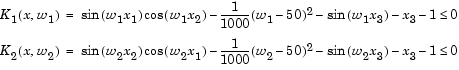
One-Dimensional Example

Find values of x that minimize

where

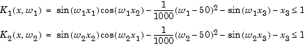
for all values of and over the ranges

Note that the semi-infinite constraints are one-dimensional, that is, vectors. Since the constraints must be in the form you need to compute the constraints as

First, write an M-file that computes the objective function.

function f = myfun(x,s)
% Objective function
f = sum((x-0.5).^2);

Second, write an M-file, mycon.m, that computes the nonlinear equality and inequality constraints and the semi-infinite constraints.

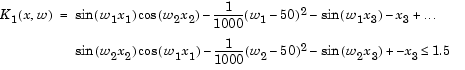
function [c,ceq,K1,K2,s] = mycon(X,s)
% Initial sampling interval
if isnan(s(1,1)),
   s = [0.2 0; 0.2 0];
end
% Sample set
w1 = 1:s(1,1):100;
w2 = 1:s(2,1):100;

% Semi-infinite constraints 
K1 = sin(w1*X(1)).*cos(w1*X(2)) - 1/1000*(w1-50).^2 -...
       sin(w1*X(3))-X(3)-1;
K2 = sin(w2*X(2)).*cos(w2*X(1)) - 1/1000*(w2-50).^2 -...
       sin(w2*X(3))-X(3)-1;

% No finite nonlinear constraints
c = []; ceq=[];

% Plot a graph of semi-infinite constraints
plot(w1,K1,'-',w2,K2,':'),title('Semi-infinite constraints')
drawnow

Then, invoke an optimization routine.

x0 = [0.5; 0.2; 0.3];      % Starting guess
[x,fval] = fseminf(@myfun,x0,2,@mycon)

After eight iterations, the solution is

The function value and the maximum values of the semi-infinite constraints at the solution x are

fval =
     0.0770

[c,ceq,K1,K2] = mycon(x,NaN);  % Use initial sampling interval
max(K1)
ans =
     -0.0017
max(K2)
ans =
     -0.0845

A plot of the semi-infinite constraints is produced.

This plot shows how peaks in both constraints are on the constraint boundary.

The plot command inside of 'mycon.m' slows down the computation. Remove this line to improve the speed.

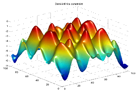
Two-Dimensional Example

Find values of x that minimize

where

for all values of and over the ranges

starting at the point .

Note that the semi-infinite constraint is two-dimensional, that is, a matrix.

First, write an M-file that computes the objective function.

function f = myfun(x,s)
% Objective function
f = sum((x-0.2).^2);

Second, write an M-file for the constraints, called mycon.m. Include code to draw the surface plot of the semi-infinite constraint each time mycon is called. This enables you to see how the constraint changes as X is being minimized.

function [c,ceq,K1,s] = mycon(X,s)
% Initial sampling interval
if isnan(s(1,1)),
   s = [2 2];
end

% Sampling set
w1x = 1:s(1,1):100;
w1y = 1:s(1,2):100;
[wx,wy] = meshgrid(w1x,w1y);

% Semi-infinite constraint 
K1 = sin(wx*X(1)).*cos(wx*X(2))-1/1000*(wx-50).^2 -...
       sin(wx*X(3))-X(3)+sin(wy*X(2)).*cos(wx*X(1))-...
       1/1000*(wy-50).^2-sin(wy*X(3))-X(3)-1.5;

% No finite nonlinear constraints
c = []; ceq=[];

% Mesh plot
m = surf(wx,wy,K1,'edgecolor','none','facecolor','interp');
camlight headlight
title('Semi-infinite constraint')
drawnow

Next, invoke an optimization routine.

x0 = [0.25, 0.25, 0.25];    % Starting guess
[x,fval] = fseminf(@myfun,x0,1,@mycon)

After nine iterations, the solution is

```
x =
     0.2926    0.1874    0.2202
```

and the function value at the solution is

```
fval = 
     0.0091
```

The goal was to minimize the objective such that the semi-infinite constraint satisfied . Evaluating mycon at the solution x and looking at the maximum element of the matrix K1 shows the constraint is easily satisfied.

[c,ceq,K1] = mycon(x,[0.5,0.5]);  % Sampling interval 0.5
max(max(K1))

ans =
    -0.0027

This call to mycon produces the following surf plot, which shows the semi-infinite constraint at x.

Algorithm

fseminf uses cubic and quadratic interpolation techniques to estimate peak values in the semi-infinite constraints. The peak values are used to form a set of constraints that are supplied to an SQP method as in the function fmincon. When the number of constraints changes, Lagrange multipliers are reallocated to the new set of constraints.

The recommended sampling interval calculation uses the difference between the interpolated peak values and peak values appearing in the data set to estimate whether more or fewer points need to be taken. The effectiveness of the interpolation is also taken into consideration by extrapolating the curve and comparing it to other points in the curve. The recommended sampling interval is decreased when the peak values are close to constraint boundaries, i.e., zero.

See also SQP Implementation for more details on the algorithm used and the types of procedures printed under the Procedures heading when the Display parameter is set to 'iter'with optimset.

Limitations

The function to be minimized, the constraints, and semi-infinite constraints, must be continuous functions of x and w. fseminf may only give local solutions.

When the problem is not feasible, fseminf attempts to minimize the maximum constraint value.

See Also

@ (function_handle), fmincon, optimset

fminunc fsolve