Getting Started

Model Order Reduction

You can derive reduced-order models with the following commands.

Model Order Reduction
balreal	Input/output balancing
minreal	Minimal realization (pole/zero cancellation)
modred	State deletion in I/O balanced realization
sminreal	Structurally minimal realization

Use minreal to delete uncontrollable or unobservable state dynamics in state-space models, or cancel pole/zero pairs in transfer functions or zero-pole-gain models. Use sminreal to remove any states that are structurally decoupled from the inputs or outputs. For already minimal models, you can further reduce the model order using a combination of balreal and modred.

Example: Gasifier Model

This example presents a model of a gasifier, a device that converts solid materials into gases. The original model is nonlinear. To load a linearized version of the model, type

• load ltiexamples
  

at the MATLAB prompt; the gasifier example is stored in the variable named gasf. If you type

• size(gasf)
  

MATLAB responds with

• State-space model with 4 outputs, 6 inputs, and 25 states.
  

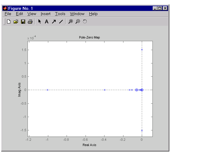
Before attempting model order reduction, inspect the pole and zero locations by using pzmap(gasf) and then zooming in near the origin. If you don't know how to use the zoom feature on plots, see Zooming for an example.

This figure shows the results.

Figure 2-5: Pole-Zero Map of the Gasifier Model (Zoomed In)

Since the model displays near pole-zero cancellations, it is a good candidate for model reduction.

SISO Model Order Reduction

As an illustration of the model order reduction tools, this example focuses on a single input/output pair of the gasifier, input 5 to output 3.

• sys35 = gasf(3,5);
  

To enhance the numerical stability, first scale the system realization with ssbal.

• sys1 = ssbal(sys35);
  

Then use minreal to eliminate uncontrollable or unobservable states.

• sys1 = minreal(sys1);
  size(sys1)
  

MATLAB responds with

• State-space model with 1 output, 1 input, and 15 states.
  

The result is a 15th order system. Use this command

• bode(sys35,sys1);
  

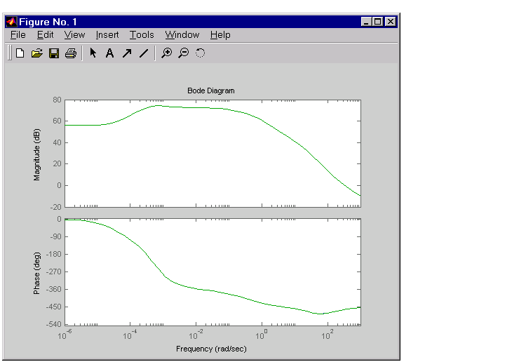
to compare the Bode magnitude and phase of the 25th order model to the reduced-order model. This figure shows the result.

Figure 2-6: Comparison of Full 25 State Model to the 15 State Reduced Order Models

As the figure shows, there is very little difference in the responses.

Finally, try eliminating states that are weakly affecting the I/O map by using the balreal and modred functions. First, attempt a balanced realization.

• [sys1,G] = balreal(sys1);
  

Use format short e to view the Hankel singular values stored in variable G.

• G =
  
    4.5468e+003
    2.6009e+003
    1.8601e+003
    2.5140e+002
    1.5081e+002
    1.1993e+001
    1.1524e+001
    1.0940e+001
    2.8766e+000
    1.3706e+000
    3.5426e-001
    2.2556e-002
    1.2496e-002
    1.0725e-002
    6.2703e-005
  

Small Hankel singular values indicate that the associated states are weakly coupled. You can try discarding the last five states (associated with the five smallest Hankel singular values).

• sys2 = modred(sys1,11:15);       % Down to 10 states
  size(sys2)
  

MATLAB responds with

• State-space model with 1 output, 1 input, and 10 states.
  

Type

• bode(sys35,sys2);
  

to compare the magnitude and phase of the 10th order model to the 25th order model.

This figure shows the result.

Figure 2-7: Comparison of 25 and 10 State Models

The figure shows good agreement until the frequency reaches 5 rad/sec. This may be acceptable since gasifiers are often low bandwidth systems, and since the models still agree at smaller frequencies. Try experimenting with discarding more Hankel values. With each further reduction, the match to the 25th order model will continue to degrade.

MIMO Model Order Reduction

You can choose not to restrict yourself to individual input/output pairs. The following code does model order reduction on the full MIMO gasifier model.

• sys1 = ssbal(gasf)      % Scaling
  
  % Compute the minimal realization and balance the model
  sys2 = minreal(sys1);    % Down to 17 states
  [sys3,G] = balreal(sys2);
  % Discard smallest entry of G by using modred
  sys3 = modred(sys3,17);    % Down to 16 states
  

After you get to 16 states, the reduced-order MIMO model begins to deteriorate when compared to the full 25 state MIMO model. Try reducing the model further to see which channels suffer the most degradation.

The MathWorks would like to thank ALSTOM Power UK for kindly permitting us to use their gasifier model for this example. This model was issued as part of the ALSTOM Benchmark Challenge on Gasifier Control. For more details see Dixon, R., (1999), "Advanced Gasifier Control," Computing & Control Engineering Journal, IEE, Vol. 10, No. 3, pp. 92-96.

Continuous/Discrete Conversions

Analyzing Models