
| Function Reference |   |
Compute the impulse response of LTI models
Syntax
impulse(sys)
impulse(sys,t)

impulse(sys1,sys2,...,sysN)
impulse(sys1,sys2,...,sysN,t)
impulse(sys1,'PlotStyle1',...,sysN,'PlotStyleN')

[y,t,x] = impulse(sys)
Description
impulse
calculates the unit impulse response of a linear system. The impulse response is the response to a Dirac input  for continuous-time systems and to a unit pulse at
  for discrete-time systems. Zero initial state is assumed in the state-space case. When invoked without left-hand arguments, this function plots the impulse response on the screen.
impulse(sys)
plots the impulse response of an arbitrary LTI model sys. This model can be continuous or discrete, and SISO or MIMO. The impulse response of multi-input systems is the collection of impulse responses for each input channel. The duration of simulation is determined automatically to display the transient behavior of the response.
impulse(sys,t)
sets the simulation horizon explicitly. You can specify either a final time t = Tfinal (in seconds), or a vector of evenly spaced time samples of the form
For discrete systems, the spacing dt should match the sample period. For continuous systems, dt becomes the sample time of the discretized simulation model (see "Algorithm"), so make sure to choose dt small enough to capture transient phenomena.
To plot the impulse responses of several LTI models sys1,..., sysN on a single figure, use
As with bode or plot, you can specify a particular color, linestyle, and/or marker for each system, for example,
See "Plotting and Comparing Multiple Systems" and the bode entry in this section for more details.
When invoked with left-side arguments,
return the output response y, the time vector t used for simulation, and the state trajectories x (for state-space models only). No plot is drawn on the screen. For single-input systems, y has as many rows as time samples (length of t), and as many columns as outputs. In the multi-input case, the impulse responses of each input channel are stacked up along the third dimension of y. The dimensions of y are then

and y(:,:,j) gives the response to an impulse disturbance entering the jth input channel. Similarly, the dimensions of x are

Example
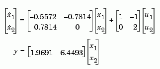
To plot the impulse response of the second-order state-space model

a = [-0.5572 -0.7814;0.7814  0];
b = [1 -1;0 2];
c = [1.9691  6.4493];
sys = ss(a,b,c,0);
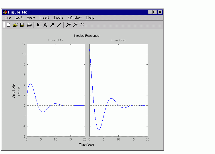
impulse(sys)
The left plot shows the impulse response of the first input channel, and the right plot shows the impulse response of the second input channel.
You can store the impulse response data in MATLAB arrays by
Because this system has two inputs, y is a 3-D array with dimensions
(the first dimension is the length of t). The impulse response of the first input channel is then accessed by
Algorithm
Continuous-time models are first converted to state space. The impulse response of a single-input state-space model

is equivalent to the following unforced response with initial state  .
.

To simulate this response, the system is discretized using zero-order hold on the inputs. The sampling period is chosen automatically based on the system dynamics, except when a time vector t = 0:dt:Tf is supplied (dt is then used as sampling period).
Limitations
The impulse response of a continuous system with nonzero  matrix is infinite at
  .
. impulse ignores this discontinuity and returns the lower continuity value  at
at  .
.
See Also
ltiview LTI system viewer
step
initial
lsim
 | hasdelay | initial |  |