
| Function Reference |   |
Syntax
step(sys)
step(sys,t)

step(sys1,sys2,...,sysN)
step(sys1,sys2,...,sysN,t)
step(sys1,'PlotStyle1',...,sysN,'PlotStyleN')

[y,t,x] = step(sys)
Description
step
calculates the unit step response of a linear system. Zero initial state is assumed in the state-space case. When invoked with no output arguments, this function plots the step response on the screen.
step(sys)
plots the step response of an arbitrary LTI model sys. This model can be continuous or discrete, and SISO or MIMO. The step response of multi-input systems is the collection of step responses for each input channel. The duration of simulation is determined automatically based on the system poles and zeros.
step(sys,t)
sets the simulation horizon explicitly. You can specify either a final time t = Tfinal (in seconds), or a vector of evenly spaced time samples of the form
For discrete systems, the spacing dt should match the sample period. For continuous systems, dt becomes the sample time of the discretized simulation model (see "Algorithm"), so make sure to choose dt small enough to capture transient phenomena.
To plot the step responses of several LTI models sys1,..., sysN on a single figure, use
All systems must have the same number of inputs and outputs but may otherwise be a mix of continuous- and discrete-time systems. This syntax is useful to compare the step responses of multiple systems.
You can also specify a distinctive color, linestyle, and/or marker for each system. For example,
plots the step response of sys1 with a dotted yellow line and the step response of sys2 with a green dashed line.
When invoked with output arguments,
return the output response y, the time vector t used for simulation, and the state trajectories x (for state-space models only). No plot is drawn on the screen. For single-input systems, y has as many rows as time samples (length of t), and as many columns as outputs. In the multi-input case, the step responses of each input channel are stacked up along the third dimension of y. The dimensions of y are then

and y(:,:,j) gives the response to a unit step command injected in the jth input channel. Similarly, the dimensions of x are

Example
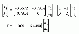
Plot the step response of the following second-order state-space model.

The left plot shows the step response of the first input channel, and the right plot shows the step response of the second input channel.
Algorithm
Continuous-time models are converted to state space and discretized using zero-order hold on the inputs. The sampling period is chosen automatically based on the system dynamics, except when a time vector t = 0:dt:Tf is supplied (dt is then used as sampling period).
See Also
impulse
initial
lsim
ltiview LTI system viewer
 | stack | tf |  |