Function Reference

initial

Compute the initial condition response of state-space models

Syntax

• initial(sys,x0)
  initial(sys,x0,t)
  
  initial(sys1,sys2,...,sysN,x0)
  initial(sys1,sys2,...,sysN,x0,t)
  initial(sys1,'PlotStyle1',...,sysN,'PlotStyleN',x0)
  
  [y,t,x] = initial(sys,x0)
  

Description

initial calculates the unforced response of a state-space model with an initial condition on the states.

This function is applicable to either continuous- or discrete-time models. When invoked without left-side arguments, initial plots the initial condition response on the screen.

initial(sys,x0) plots the response of sys to an initial condition x0 on the states. sys can be any state-space model (continuous or discrete, SISO or MIMO, with or without inputs). The duration of simulation is determined automatically to reflect adequately the response transients.

initial(sys,x0,t) explicitly sets the simulation horizon. You can specify either a final time t = Tfinal (in seconds), or a vector of evenly spaced time samples of the form

• t = 0:dt:Tfinal
  

For discrete systems, the spacing dt should match the sample period. For continuous systems, dt becomes the sample time of the discretized simulation model (see impulse), so make sure to choose dt small enough to capture transient phenomena.

To plot the initial condition responses of several LTI models on a single figure, use

• initial(sys1,sys2,...,sysN,x0) 
  initial(sys1,sys2,...,sysN,x0,t) 
  

(see impulse for details).

When invoked with left-side arguments,

• [y,t,x] = initial(sys,x0)
  [y,t,x] = initial(sys,x0,t)
  

return the output response y, the time vector t used for simulation, and the state trajectories x. No plot is drawn on the screen. The array y has as many rows as time samples (length of t) and as many columns as outputs. Similarly, x has length(t) rows and as many columns as states.

Example

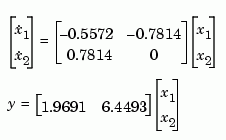
Plot the response of the state-space model

to the initial condition

• a = [-0.5572   -0.7814;0.7814  0];
  c = [1.9691  6.4493];
  x0 = [1 ; 0]
  
  sys = ss(a,[],c,[]);
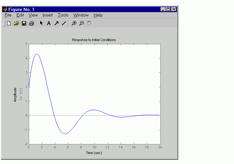
  initial(sys,x0)
  

See Also
impulse     Impulse response

lsim        Simulate response to arbitrary inputs

ltiview     LTI system viewer

step        Step response

impulse

interp