

| Function Reference | |
Specify transfer functions or convert LTI model to transfer function form
Syntax
sys = tf(num,den)
sys = tf(num,den,Ts)
sys = tf(M)
sys = tf(num,den,ltisys)

sys = tf(num,den,'Property1',Value1,...,'PropertyN',ValueN)
sys = tf(num,den,Ts,'Property1',Value1,...,'PropertyN',ValueN)

sys = tf('s')
sys = tf('z')

tfsys = tf(sys)
tfsys = tf(sys,'inv')    % for state-space sys only
Description
tf
is used to create real- or complex-valued transfer function models (TF objects) or to convert state-space or zero-pole-gain models to transfer function form.
Creation of Transfer Functions
sys = tf(num,den)
creates a continuous-time transfer function with numerator(s) and denominator(s) specified by num and den. The output sys is a TF object storing the transfer function data (see "Transfer Function Models" on page 2-8).
In the SISO case, num and den are the real- or complex-valued row vectors of numerator and denominator coefficients ordered in descending powers of  . These two vectors need not have equal length and the transfer function need not be proper. For example,
 h = tf([1 0],1) specifies the pure derivative  .
.
To create MIMO transfer functions, specify the numerator and denominator of each SISO entry. In this case:
num and den are cell arrays of row vectors with as many rows as outputs and as many columns as inputs.
num{i,j} and den{i,j} specify the numerator and denominator of the transfer function from input j to output i (with the SISO convention).
If all SISO entries of a MIMO transfer function have the same denominator, you can set den to the row vector representation of this common denominator. See "Examples" for more details.
sys = tf(num,den,Ts)
creates a discrete-time transfer function with sample time Ts (in seconds). Set Ts = -1 or Ts = [] to leave the sample time unspecified. The input arguments num and den are as in the continuous-time case and must list the numerator and denominator coefficients in descending powers of  .
.
sys = tf(M)
creates a static gain M (scalar or matrix).
sys = tf(num,den,ltisys)
creates a transfer function with generic LTI properties inherited from the LTI model ltisys (including the sample time). See "Generic Properties" on page 2-26 for an overview of generic LTI properties.
There are several ways to create LTI arrays of transfer functions. To create arrays of SISO or MIMO TF models, either specify the numerator and denominator of each SISO entry using multidimensional cell arrays, or use a for loop to successively assign each TF model in the array. See "Building LTI Arrays" on page 4-12 for more information.
Any of the previous syntaxes can be followed by property name/property value pairs
Each pair specifies a particular LTI property of the model, for example, the input names or the transfer function variable. See set entry and the example below for details. Note that
Transfer Functions as Rational Expressions in s or z
You can also use real- or complex-valued rational expressions to create a TF model. To do so, first type either:
s = tf('s') to specify a TF model using a rational function in the Laplace variable, s.
z = tf('z',Ts) to specify a TF model with sample time Ts using a rational function in the discrete-time variable, z.
Once you specify either of these variables, you can specify TF models directly as rational expressions in the variable s or z by entering your transfer function as a rational expression in either s or z.
Conversion to Transfer Function
tfsys = tf(sys)
converts an arbitrary SS or ZPK LTI model sys to transfer function form. The output tfsys (TF object) is the transfer function of sys. By default, tf uses zero to compute the numerators when converting a state-space model to transfer function form. Alternatively,
uses inversion formulas for state-space models to derive the numerators. This algorithm is faster but less accurate for high-order models with low gain at  .
.
Example 1
Create the two-output/one-input transfer function
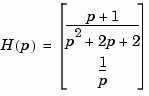
with input current and outputs torque and ang velocity.
num = {[1 1] ; 1}
den = {[1 2 2] ; [1 0]}
H = tf(num,den,'inputn','current',...
                    'outputn',{'torque' 'ang. velocity'},...
                    'variable','p')
Transfer function from input "current" to output...
              p + 1
 torque:  -------------
          p^2 + 2 p + 2

                 1
 ang. velocity:  -
                 p
Note how setting the 'variable' property to 'p' causes the result to be displayed as a transfer function of the variable  .
.
Example 2
To use a rational expression to create a SISO TF model, type
This produces the same transfer function as
Example 3
Specify the discrete MIMO transfer function
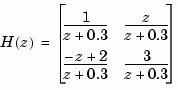
with common denominator 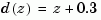 and sample time of 0.2 seconds.
Example 4
Compute the transfer function of the state-space model with the following data.
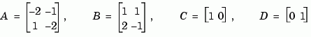
sys = ss([-2 -1;1 -2],[1 1;2 -1],[1 0],[0 1])
tf(sys)
Transfer function from input 1 to output:
      s
-------------
s^2 + 4 s + 5

Transfer function from input 2 to output:
s^2 + 5 s + 8
-------------
s^2 + 4 s + 5
You can use a for loop to specify a 10-by-1 array of SISO TF models.
The first statement pre-allocates the TF array and fills it with zero transfer functions.
Discrete-Time Conventions
The control and digital signal processing (DSP) communities tend to use different conventions to specify discrete transfer functions. Most control engineers use the  variable and order the numerator and denominator terms in descending powers of
  , for example,
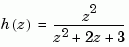
The polynomials  and
and  are then specified by the row vectors
 [1 0 0] and [1 2 3], respectively. By contrast, DSP engineers prefer to write this transfer function as
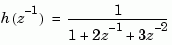
and specify its numerator as 1 (instead of [1 0 0]) and its denominator as [1 2 3].
tf switches convention based on your choice of variable (value of the 'Variable' property).
specifies the discrete transfer function
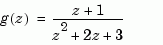
because  is the default variable. In contrast,
uses the DSP convention and creates
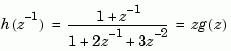
See also filt for direct specification of discrete transfer functions using the DSP convention.
Note that tf stores data so that the numerator and denominator lengths are made equal. Specifically, tf stores the values
for g (the numerator is padded with zeros on the left) and the values
for h (the numerator is padded with zeros on the right).
Algorithm
tf uses the MATLAB function poly to convert zero-pole-gain models, and the functions zero and pole to convert state-space models.
See Also
filt
frd Specify a frequency response data model
get Get properties of LTI models
set Set properties of LTI models
ss Specify state-space models or convert to state space
tfdata
zpk Specify zero-pole-gain models or convert to ZPK
| | step | tfdata | |
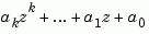 (coefficients ordered in descending powers of
  ).
).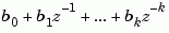 (coefficients in ascending powers of
  or
or  ).
).