
| Function Reference |   |
Compute Nyquist frequency response of LTI models
Syntax
nyquist(sys)
nyquist(sys,w)

nyquist(sys1,sys2,...,sysN)
nyquist(sys1,sys2,...,sysN,w)
nyquist(sys1,'PlotStyle1',...,sysN,'PlotStyleN')

[re,im,w] = nyquist(sys)
[re,im] = nyquist(sys,w)
Description
nyquist
calculates the Nyquist frequency response of LTI models. When invoked without left-hand arguments, nyquist produces a Nyquist plot on the screen. Nyquist plots are used to analyze system properties including gain margin, phase margin, and stability.
nyquist(sys)
plots the Nyquist response of an arbitrary LTI model sys. This model can be continuous or discrete, and SISO or MIMO. In the MIMO case, nyquist produces an array of Nyquist plots, each plot showing the response of one particular I/O channel. The frequency points are chosen automatically based on the system poles and zeros.
nyquist(sys,w explicitly specifies the frequency range or frequency points to be used for the plot. To focus on a particular frequency interval, set )
w = {wmin,wmax}. To use particular frequency points, set w to the vector of desired frequencies. Use logspace to generate logarithmically spaced frequency vectors. Frequencies should be specified in rad/sec.
nyquist(sys1,sys2,...,sysN) or nyquist(sys1,sys2,...,sysN,w) superimposes the Nyquist plots of several LTI models on a single figure. All systems must have the same number of inputs and outputs, but may otherwise be a mix of continuous- and discrete-time systems. You can also specify a distinctive color, linestyle, and/or marker for each system plot with the syntax
When invoked with left-hand arguments
return the real and imaginary parts of the frequency response at the frequencies w (in rad/sec). re and im are 3-D arrays (see "Arguments" below for details).
Arguments
The output arguments re and im are 3-D arrays with dimensions

For SISO systems, the scalars re(1,1,k) and im(1,1,k) are the real and imaginary parts of the response at the frequency  .
.

For MIMO systems with transfer function  ,
, re(:,:,k) and im(:,:,k) give the real and imaginary parts of  (both arrays with as many rows as outputs and as many columns as inputs). Thus,

where  is the transfer function from input
  to output
  .
.
Example
Plot the Nyquist response of the system

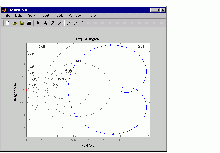
The nyquist function has support for M-circles, which are the contours of the constant closed-loop magnitude. M-circles are defined as the locus of complex numbers where

is a constant value. In this equation,  is the frequency in radians/second, and G is the collection of complex numbers that satisfy the constant magnitude requirement.
To activate the grid, select Grid from the right-click menu or type
at the MATLAB prompt. This figure shows the M circles for transfer function H.
You have two zoom options available from the right-click menu that apply specifically to Nyquist plots:
Also, click anywhere on the curve to activate data markers that display the real and imaginary values at a given frequency. This figure shows the nyquist plot with a data marker.
See Also
bode Bode plot
evalfr Response at single complex frequency
freqresp Frequency response computation
ltiview LTI system viewer
nichols Nichols plot
sigma Singular value plot
 | norm | obsv |  |