lsim (Function Reference)

Simulate LTI model response to arbitrary inputs

Syntax

lsim(sys,u,t)
lsim(sys,u,t,x0)
lsim(sys,u,t,x0,'zoh')
lsim(sys,u,t,x0,'foh') 

lsim(sys1,sys2,...,sysN,u,t)
lsim(sys1,sys2,...,sysN,u,t,x0)
lsim(sys1,'PlotStyle1',...,sysN,'PlotStyleN',u,t)

[y,t,x] = lsim(sys,u,t,x0)

Description

lsim simulates the (time) response of continuous or discrete linear systems to arbitrary inputs. When invoked without left-hand arguments, lsim plots the response on the screen.

lsim(sys,u,t) produces a plot of the time response of the LTI model sys to the input time history t,u. The vector t specifies the time samples for the simulation and consists of regularly spaced time samples.

```
t = 0:dt:Tfinal
```

The matrix u must have as many rows as time samples (length(t)) and as many columns as system inputs. Each row u(i,:) specifies the input value(s) at the time sample t(i).

The LTI model sys can be continuous or discrete, SISO or MIMO. In discrete time, u must be sampled at the same rate as the system (t is then redundant and can be omitted or set to the empty matrix). In continuous time, the time sampling dt=t(2)-t(1) is used to discretize the continuous model. If dt is too large (undersampling), lsim issues a warning suggesting that you use a more appropriate sample time, but will use the specified sample time. See Algorithm for a discussion of sample times.

lsim(sys,u,t,x0) further specifies an initial condition x0 for the system states. This syntax applies only to state-space models.

lsim(sys,u,t,x0,'zoh') or lsim(sys,u,t,x0,'foh') explicitly specifies how the input values should be interpolated between samples (zero-order hold or linear interpolation). By default, lsim selects the interpolation method automatically based on the smoothness of the signal U.

Finally,

```
lsim(sys1,sys2,...,sysN,u,t) 
```

simulates the responses of several LTI models to the same input history t,u and plots these responses on a single figure. As with bode or plot, you can specify a particular color, linestyle, and/or marker for each system, for example,

```
lsim(sys1,'y:',sys2,'g--',u,t,x0)
```

The multisystem behavior is similar to that of bode or step.

When invoked with left-hand arguments,

[y,t] = lsim(sys,u,t)
[y,t,x] = lsim(sys,u,t)        % for state-space models only
[y,t,x] = lsim(sys,u,t,x0)     % with initial state

return the output response y, the time vector t used for simulation, and the state trajectories x (for state-space models only). No plot is drawn on the screen. The matrix y has as many rows as time samples (length(t)) and as many columns as system outputs. The same holds for x with "outputs" replaced by states. Note that the output t may differ from the specified time vector when the input data is undersampled (see Algorithm).

Example

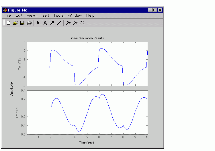
Simulate and plot the response of the system

to a square wave with period of four seconds. First generate the square wave with gensig. Sample every 0.1 second during 10 seconds:

```
[u,t] = gensig('square',4,10,0.1);
```

Then simulate with lsim.

H = [tf([2 5 1],[1 2 3]) ; tf([1 -1],[1 1 5])]
lsim(H,u,t)

Algorithm

Discrete-time systems are simulated with ltitr (state space) or filter (transfer function and zero-pole-gain).

Continuous-time systems are discretized with c2d using either the 'zoh' or 'foh' method ('foh' is used for smooth input signals and 'zoh' for discontinuous signals such as pulses or square waves). The sampling period is set to the spacing dt between the user-supplied time samples t.

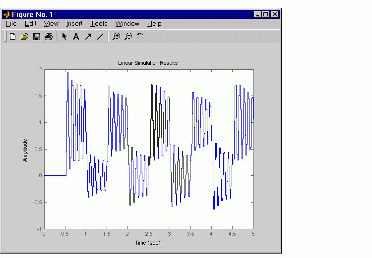
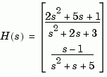
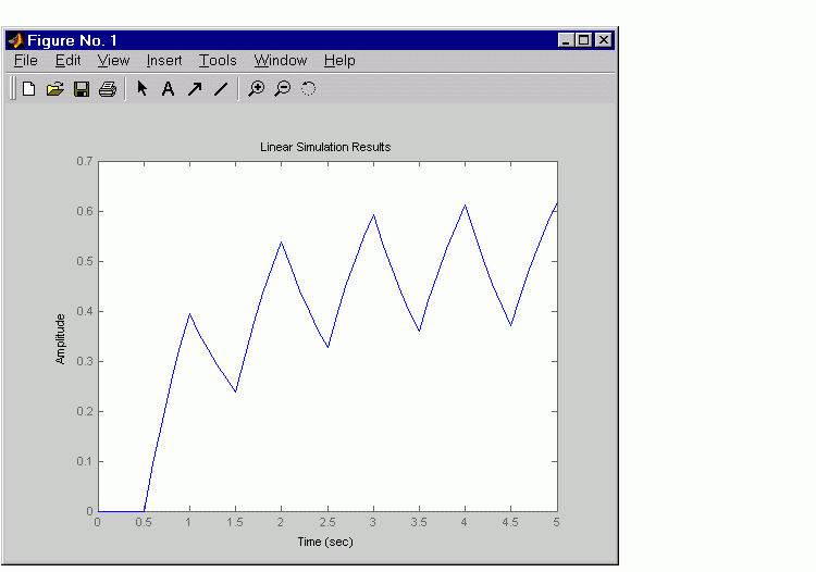
The choice of sampling period can drastically affect simulation results. To illustrate why, consider the second-order model

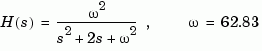
To simulate its response to a square wave with period 1 second, you can proceed as follows:

w2 = 62.83^2
h = tf(w2,[1 2 w2])
t = 0:0.1:5;             % vector of time samples
u = (rem(t,1)>=0.5);   % square wave values
lsim(h,u,t)

lsim evaluates the specified sample time, gives this warning

Warning: Input signal is undersampled. Sample every 0.016 sec or 
faster.

and produces this plot.

To improve on this response, discretize using the recommended sampling period:

dt=0.016;
ts=0:dt:5;
us = (rem(ts,1)>=0.5)
hd = c2d(h,dt)
lsim(hd,us,ts)

This response exhibits strong oscillatory behavior hidden from the undersampled version.

See Also
gensig Generate test input signals for lsim

impulse Impulse response

initial Free response to initial condition

ltiview LTI system viewer

step Step response

lqry ltimodels