

| Getting Started |   |
Example: LQG Design for Set Point Tracking
The standard LQG problem is to regulate the plant output around zero. The previous section, Example: LQG Design, describes the classical LQG regulation problem.
You can also apply the LQG design technique to tracking problems, where the goal is to track a reference input (or set point) to the system. To recast the regulator as a tracking problem, you must compare the output y to the reference signal. The goal is then to drive the error between the output and the reference to zero. A common practice is to add an integrator to the error signal, e = y - r, to drive it to zero.
This Simulink block diagram shows a tracking problem in aircraft autopilot design. To open this diagram, type lqrpilot at the MATLAB prompt.
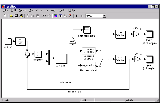
Key features of this diagram to note are the following:
sf_aerodyn is an S-Function block that contains the nonlinear equations for 
 and the
  is passed through an integrator. This aids in driving the error to zero.
State-Space Equations for an Airframe
Beginning with the standard state-space equation
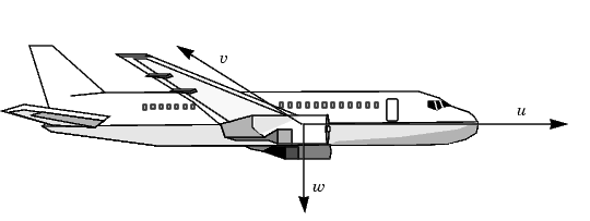
The variables u, v, and w are the three velocities with respect to the body frame, which is shown in the figure below
 .
.
Figure 4-55: A Body Coordinate Frame for an Aircraft
The variables  and
and  are roll and pitch, and p, q, and r are the roll, pitch, and yaw rates, respectively.
The airframe dynamics are nonlinear. The equation below shows the nonlinear components added to the state space equation.
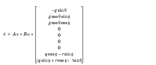
Figure 4-56: Nonlinear Component of the State-Space Equation
To see the numerical values for A and B, type
Trimming
For LQG design purposes, the nonlinear dynamics are trimmed at  and p, q, r, and
  set to zero. Since u, v, and w do not enter into the nonlinear term in Figure 4-56, this amounts to linearizing around
  with all remaining states set to zero. The resulting state matrix of the linearized model is called
 A15.
Problem Definition
The goal to perform a steady coordinated turn, as shown in this figure.

Figure 4-57: An Aircraft Making a 60° Turn
To achieve this goal, you must design a controller that commands a steady turn by going through a 60° roll. In addition, assume that  , the pitch angle, is required to stay as close to zero as possible.
Results
To calculate the LQG gain matrix, K, type
at the MATLAB prompt. Then start the lqrpilot model with the nonlinear model, sf_aerodyn, selected. This figure shows the response of  to the 60° step command.
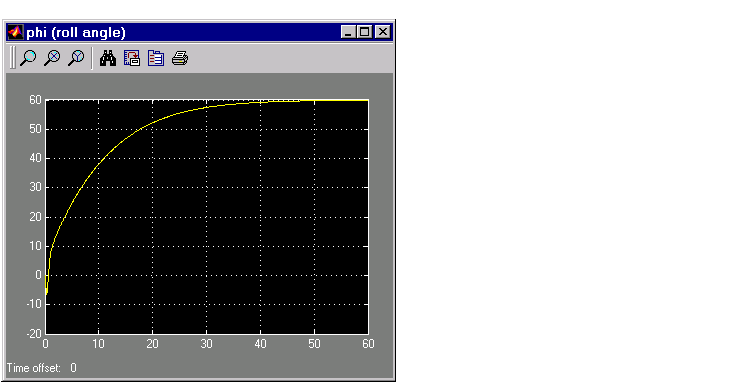
Figure 4-58: Tracking the Roll Step Command
As you can see, the system tracks the commanded 60° roll in about 60 seconds.
Another goal was to keep  , the pitch angle, relatively small. This figure shows how well the LQG controller did.
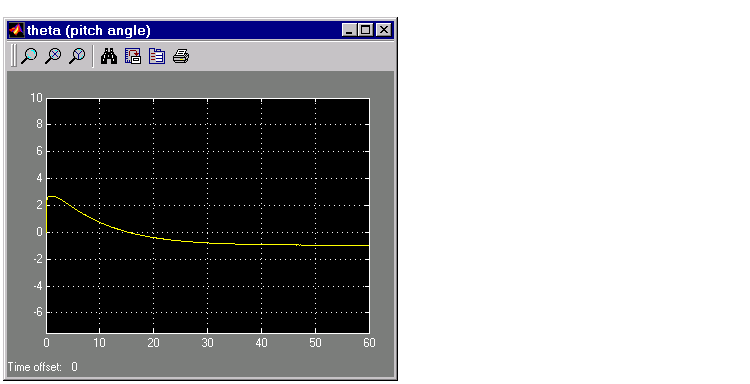
Figure 4-59: Minimizing the Displacement in the Pitch Angle, Theta
Finally, this figure shows the control inputs.
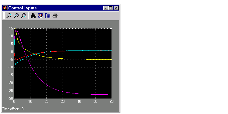
Figure 4-60: The Control Inputs for the LQG Tracking Problem
Try adjusting the Q and R matrices in lqrdes.m and inspecting the control inputs and the system states, making sure to rerun lqrdes to update the LQG gain matrix K. Through trial and error, you may improve the response time of this design. Also, compare the linear and nonlinear designs to see the effects of the nonlinearities on the system performance.
 | Example: LQG Design | Learning More |  |