
| System Identification Toolbox |   |
Choosing an Adaptation Mechanism and Gain
The most logical approach to the adaptation problem is to assume a certain model for how the "true" parameters  change. A typical choice is to describe these parameters as a random walk.

|
(3-58) |
Here  is assumed to be white Gaussian noise with covariance matrix

|
(3-59) |
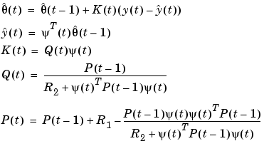
Suppose that the underlying description of the observations is a linear regression (3-57). An optimal choice of  in (3-55)-(3-56) can then be computed from the Kalman filter, and the complete algorithm becomes

|
(3-60) |
Here  is the variance of the innovations
  in (3-57):
  (a scalar). The algorithm (3-60) will be called the Kalman filter (KF) approach to adaptation, with drift matrix
  . See eq (11.66)-(11.67) in Ljung (1999). The algorithm is entirely specified by
 ,
, ,
, ,
, , and the sequence of data
  ,
, ,
,  , 2,.... Even though the algorithm was motivated for a linear regression model structure, it can also be applied in the general case where
  is computed in a different way from (3-60b).
Another approach is to discount old measurements exponentially, so that an observation that is  samples old carries a weight that is
  of the weight of the most recent observation. This means that the following function is minimized rather than (3-39)

|
(3-61) |
at time t. Here  is a positive number (slightly) less than 1. The measurements that are older than
  carry a weight in the expression above that is less than about 0.3. Think of
  as the memory horizon of the approach. Typical values of
  are in the range 0.97- 0.995.
The criterion (3-61) can be minimized exactly in the linear regression case giving the algorithm (3-60abc) with the following choice of  .
.

|
(3-62) |
This algorithm will be called the Forgetting Factor (FF) approach to adaptation, with the forgetting factor  . See eq (11.63) in Ljung (1999). The algorithm is also known as recursive least squares (RLS) in the linear regression case. Note that
  in this approach gives the same algorithm as
  in the Kalman filter approach.
A third approach is to allow the matrix  to be a multiple of the identity matrix.

|
(3-63) |
It can also be normalized with respect to the size of  .
.

|
(3-64) |
See eqs (11.45) and (11.46), respectively in Ljung (1999). These choices of  move the updates of
  in (3-55) in the negative gradient direction (with respect to
  ) of the criterion (3-39). Therefore, (3-63) will be called the Unnormalized Gradient (UG) approach and (3-64) the Normalized Gradient (NG) approach to adaptation, with gain
  . The gradient methods are also known as least mean squares (LMS) in the linear regression case.
 | The Basic Algorithm | Available Algorithms |  |