Optimization Toolbox

Constrained Example with Gradients

Ordinarily the medium-scale minimization routines use numerical gradients calculated by finite-difference approximation. This procedure systematically perturbs each of the variables in order to calculate function and constraint partial derivatives. Alternatively, you can provide a function to compute partial derivatives analytically. Typically, the problem is solved more accurately and efficiently if such a function is provided.

To solve Eq. 2-2 using analytically determined gradients, do the following.

Step 1: Write an M-file for the objective function and gradient.

• function [f,G] = objfungrad(x)
  f = exp(x(1))*(4*x(1)^2+2*x(2)^2+4*x(1)*x(2)+2*x(2)+1);
  % Gradient of the objective function
  t = exp(x(1))*(4*x(1)^2+2*x(2)^2+4*x(1)*x(2)+2*x(2)+1);
  G = [ t + exp(x(1)) * (8*x(1) + 4*x(2)), 
      exp(x(1))*(4*x(1)+4*x(2)+2)];
  

Step 2: Write an M-file for the nonlinear constraints and the gradients of the nonlinear constraints.

• function [c,ceq,DC,DCeq] = confungrad(x)
  c(1) = 1.5 + x(1) * x(2) - x(1) - x(2);   %Inequality constraints
  c(2) = -x(1) * x(2)-10; 
  % Gradient of the constraints
  DC= [x(2)-1, -x(2);
        x(1)-1, -x(1)];
  % No nonlinear equality constraints
  ceq=[];
  DCeq = [ ];
  

G contains the partial derivatives of the objective function, f, returned by objfungrad(x), with respect to each of the elements in x:

(2-4)

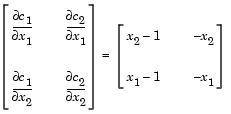
The columns of DC contain the partial derivatives for each respective constraint (i.e., the ith column of DC is the partial derivative of the ith constraint with respect to x). So in the above example, DC is

(2-5)

Since you are providing the gradient of the objective in objfungrad.m and the gradient of the constraints in confungrad.m, you must tell fmincon that these M-files contain this additional information. Use optimset to turn the parameters GradObj and GradConstr to 'on' in the example's existing options structure:

• options = optimset(options,'GradObj','on','GradConstr','on');
  

If you do not set these parameters to 'on' in the options structure, fmincon does not use the analytic gradients.

The arguments lb and ub place lower and upper bounds on the independent variables in x. In this example, there are no bound constraints and so they are both set to [].

Step 3: Invoke constrained optimization routine.

• x0 = [-1,1];            % Starting guess 
  options = optimset('LargeScale','off');
  options = optimset(options,'GradObj','on','GradConstr','on');
  lb = [ ]; ub = [ ];   % No upper or lower bounds
  [x,fval] = fmincon(@objfungrad,x0,[],[],[],[],lb,ub,... 
     @confungrad,options)
  [c,ceq] = confungrad(x) % Check the constraint values at x
  

After 20 function evaluations, the solution produced is

• x =
      -9.5474    1.0474
  fval =
       0.0236
  c =
       1.0e-14 *
       0.1110
      -0.1776
  ceq =
       []
  

Constrained Example with Bounds

Gradient Check: Analytic Versus Numeric