

| Creating and Manipulating Models | |
State-Space Models
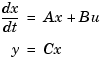
State-space models rely on linear differential or difference equations to describe the system dynamics. Continuous-time models are of the form
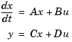
where x is the state vector and u and y are the input and output vectors. Such models may arise from the equations of physics, from state-space identification, or by state-space realization of the system transfer function.
Use the command ss to create state-space models
For a model with Nx states, Ny outputs, and Nu inputs
A is an Nx-by-Nx real-valued matrix.
B is an Nx-by-Nu real-valued matrix.
C is an Ny-by-Nx real-valued matrix.
D is an Ny-by-Nu real-valued matrix.
This produces an SS object sys that stores the state-space matrices  . For models with a zero D matrix, you can use
 D = 0 (zero) as a shorthand for a zero matrix of the appropriate dimensions.
As an illustration, consider the following simple model of an electric motor.
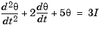
where  is the angular displacement of the rotor and
  the driving current. The relation between the input current
  and the angular velocity
  is described by the state-space equations
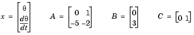
This model is specified by typing
a =
                        x1           x2
           x1            0      1.00000
           x2     -5.00000     -2.00000

b =
                        u1
           x1            0
           x2      3.00000

c =
                        x1           x2
           y1            0      1.00000

d =
                        u1
           y1            0
In addition to the A, B, C, and D matrices, the display of state-space models includes state names, input names, and output names. Default names (here, x1, x2, u1, and y1) are displayed whenever you leave these unspecified. See LTI Properties for more information on how to specify state, input, or output names.
| | Zero-Pole-Gain Models | Descriptor State-Space Models | |