Statistics Toolbox

Regression and Classification Trees

In nonlinear least squares we suppose that we know the form of the relationship between the response and predictor. Suppose instead that we don't know that relationship, and also that we are unwilling to assume the relationship can be well approximated by a linear model. We need a more nonparametric type of regression fitting approach. One such approach is based on "trees."

A regression tree is a sequence of questions that can be answered as yes or no, plus a set of fitted response values. Each question asks whether a predictor satisfies a given condition. Predictors can be continuous or discrete. Depending on the answers to one question, we either proceed to another question or we arrive at a fitted response value.

In this example we fit a regression tree to variables from the carsmall data set. We use the same variables as in the Analysis of Covariance example (see The aoctool Demo), so we have one continuous predictor (car weight) and one discrete predictor (model year).

Our goal is to model mileage (MPG) as a function of car weight and model year. First we load the data and then create a matrix x of predictor values and a vector y of response variables. We fit a regression tree, specifying the model year column as a categorical variable. In this data set there are cars from the three different model years 1970, 1976, and 1982.

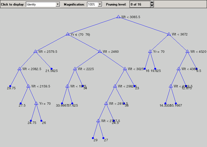
• load carsmall
  x = [Weight,Model_Year];
  y = MPG;
  t = treefit(x,y,'catidx',2);
  treedisp(t,'name',{'Wt' 'Yr'});
  
  
  

Now we want to use this model to determine the predicted mileage for a car weighing 3000 pounds from model year 1982. Start at the top node. The weight is less than the cutoff value of 3085.5, so we take the left branch. The model year is not 1970 or 1976, so we take the right branch. We continue moving down the tree until we arrive at a terminal node that gives the predicted value. In this case, the predicted value is 38 miles per gallon. We can use the treeval function to find the fitted value for any set of predictor values.

• treeval(t,[3000 82])
  
  ans =
      38
  

With a tree like this one having many branches, there is a danger that it fits the current data set well but would not do a good job at predicting new values. Some of its lower branches may be strongly affected by outliers and other artifacts of the current data set. If possible we would prefer to find a simpler tree that avoids this problem of over-fitting.

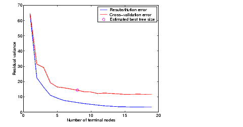
We'll estimate the best tree size by cross validation. First we compute a "resubstitution" estimate of the error variance for this tree and a sequence of simpler trees and plot it as the lower (blue) line in the figure. This estimate probably under-estimates the true error variance. Then we compute a "cross-validation" estimate of the same quantity and plot it as the upper (red) line. The cross-validation procedure also provides us with an estimate of the pruning level, best, needed to achieve the best tree size.

• [c,s,ntn] = treetest(t,'resub');
  [c2,s2,n2,best] = treetest(t,'cross',x,y);
  plot(ntn,c,'b-', n2,c2,'r-', n2(best+1),c2(best+1),'mo');
  xlabel('Number of terminal nodes')
  ylabel('Residual variance')
  legend('Resubstitution error','Cross-validation 
  error','Estimated best tree size')
  best
  
  best =
      10
  
  
  

The best tree is the one that has a residual variance that is no more than one standard error above the minimum value along the cross-validation line. In this case the variance is just over 14. The output best takes on values starting with 0 (representing no pruning), so we need to add 1 to use it as an index into the other output arguments.

• c2(best+1)
  ans =
     14.3440
  

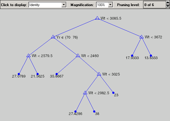
Use the output best to create a smaller tree that is pruned to our estimated best size.

• t0 = treeprune(t,'level',best);
  treedisp(t0,'name',{'Wt' 'Yr'})
  
  
  

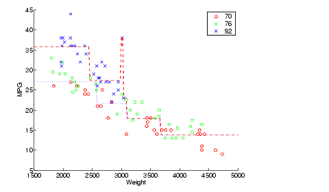
Now plot the original data and overlay the fitted values that we get using this tree. Notice that this tree does not distinguish between cars from 1970 or 1976, so we'll create a vector yold containing fitted values for 1976 and another ynew for year 1982. Cars from 1970 have the same fitted values as those from 1976.

• xx = (1500:20:5000)';
  ynew = treeval(t0,[xx 82*ones(size(xx))]);
  yold = treeval(t0,[xx 76*ones(size(xx))]);
  gscatter(Weight,MPG,Model_Year,'rgb','osx');
  hold on; plot(xx,yold,'b:', xx,ynew,'r--'); hold off
  
  
  

The tree functions (treedisp, treefit, treeprune, treetest, and treeval) can also accept a categorical response variable. In that case, the fitted value from the tree is the category with the highest predicted probability for the range of predictor values falling in a given node. The Statistics Toolbox demo entitled Classification of Fisher's Iris Data shows how to use decision trees for classification.

An Interactive GUI for Nonlinear Fitting and Prediction

Hypothesis Tests