Signal Processing Toolbox

Parametric Methods

Parametric methods can yield higher resolutions than nonparametric methods in cases when the signal length is short. These methods use a different approach to spectral estimation; instead of trying to estimate the PSD directly from the data, they model the data as the output of a linear system driven by white noise, and then attempt to estimate the parameters of that linear system.

The most commonly used linear system model is the all-pole model, a filter with all of its zeroes at the origin in the z-plane. The output of such a filter for white noise input is an autoregressive (AR) process. For this reason, these methods are sometimes referred to as AR methods of spectral estimation.

The AR methods tend to adequately describe spectra of data that is "peaky," that is, data whose PSD is large at certain frequencies. The data in many practical applications (such as speech) tends to have "peaky spectra" so that AR models are often useful. In addition, the AR models lead to a system of linear equations which is relatively simple to solve.

The Signal Processing Toolbox offers the following AR methods for spectral estimation:

• Yule-Walker AR method (autocorrelation method)
• Burg method
• Covariance method
• Modified covariance method

All AR methods yield a PSD estimate given by

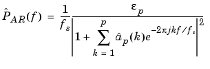
The different AR methods estimate the AR parameters a_p(k) slightly differently, yielding different PSD estimates. The following table provides a summary of the different AR methods.

	Burg	Covariance	Modified Covariance	Yule-Walker
Characteristics	Does not apply window to data	Does not apply window to data	Does not apply window to data	Applies window to data
	Minimizes the forward and backward prediction errors in the least squares sense, with the AR coefficients constrained to satisfy the L-D recursion	Minimizes the forward prediction error in the least squares sense	Minimizes the forward and backward prediction errors in the least squares sense	Minimizes the forward prediction error in the least squares sense (also called "Autocorrelation method")
Advantages	High resolution for short data records	Better resolution than Y-W for short data records (more accurate estimates)	High resolution for short data records	Performs as well as other methods for large data records
	Always produces a stable model	Able to extract frequencies from data consisting of p or more pure sinusoids	Able to extract frequencies from data consisting of p or more pure sinusoids	Always produces a stable model
			Does not suffer spectral line-splitting
Disadvantages	Peak locations highly dependent on initial phase	May produce unstable models	May produce unstable models	Performs relatively poorly for short data records
	May suffer spectral line-splitting for sinusoids in noise, or when order is very large	Frequency bias for estimates of sinusoids in noise	Peak locations slightly dependent on initial phase	Frequency bias for estimates of sinusoids in noise
	Frequency bias for estimates of sinusoids in noise		Minor frequency bias for estimates of sinusoids in noise
Conditions for Nonsingularity		Order must be less than or equal to half the input frame size	Order must be less than or equal to 2/3 the input frame size	Because of the biased estimate, the autocorrelation matrix is guaranteed to positive-definite, hence nonsingular

Yule-Walker AR Method

The Yule-Walker AR method of spectral estimation computes the AR parameters by forming a biased estimate of the signal's autocorrelation function, and solving the least squares minimization of the forward prediction error. This results in the Yule-Walker equations.

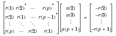
The use of a biased estimate of the autocorrelation function ensures that the autocorrelation matrix above is positive definite. Hence, the matrix is invertible and a solution is guaranteed to exist. Moreover, the AR parameters thus computed always result in a stable all-pole model. The Yule-Walker equations can be solved efficiently via Levinson's algorithm, which takes advantage of the Toeplitz structure of the autocorrelation matrix.

The toolbox function pyulear implements the Yule-Walker AR method.

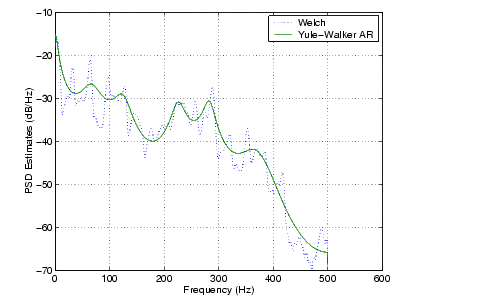
For example, compare the spectrum of a speech signal using Welch's method and the Yule-Walker AR method:

• load mtlb
  [P1,f] = pwelch(mtlb,hamming(256),128,1024,fs);
  [P2,f] = pyulear(mtlb,14,1024,fs);
  plot(f,10*log10(P1),':',f,10*log10(P2)); grid
  ylabel('PSD Estimates (dB/Hz)');
  xlabel('Frequency (Hz)');
  legend('Welch','Yule-Walker AR')
  
  
  

The solid-line Yule-Walker AR spectrum is smoother than the periodogram because of the simple underlying all-pole model.

Burg Method

The Burg method for AR spectral estimation is based on minimizing the forward and backward prediction errors while satisfying the Levinson-Durbin recursion (see Marple [3], Chapter 7, and Proakis [6], Section 12.3.3). In contrast to other AR estimation methods, the Burg method avoids calculating the autocorrelation function, and instead estimates the reflection coefficients directly.

The primary advantages of the Burg method are resolving closely spaced sinusoids in signals with low noise levels, and estimating short data records, in which case the AR power spectral density estimates are very close to the true values. In addition, the Burg method ensures a stable AR model and is computationally efficient.

The accuracy of the Burg method is lower for high-order models, long data records, and high signal-to-noise ratios (which can cause line splitting, or the generation of extraneous peaks in the spectrum estimate). The spectral density estimate computed by the Burg method is also susceptible to frequency shifts (relative to the true frequency) resulting from the initial phase of noisy sinusoidal signals. This effect is magnified when analyzing short data sequences.

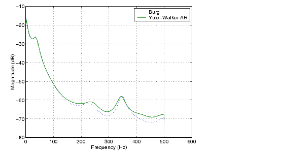
The toolbox function pburg implements the Burg method. Compare the spectrum of the speech signal generated by both the Burg method and the Yule-Walker AR method. They are very similar for large signal lengths:

• load mtlb
  [P1,f] = pburg(mtlb(1:512),14,1024,fs);% 14th order model
  [P2,f] = pyulear(mtlb(1:512),14,1024,fs);% 14th order model
  plot(f,10*log10(P1),':',f,10*log10(P2)); grid
  ylabel('Magnitude (dB)'); xlabel('Frequency (Hz)');
  legend('Burg','Yule-Walker AR')
  
  
  

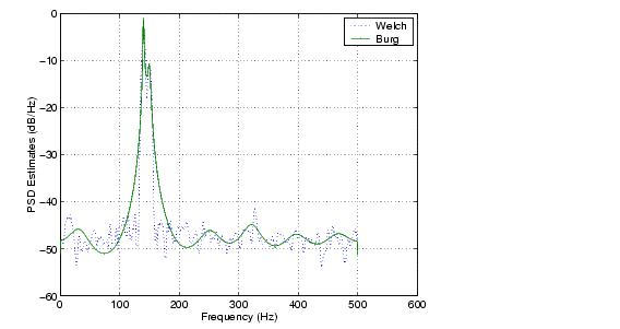
Compare the spectrum of a noisy signal computed using the Burg method and the Welch method:

• randn('state',0)
  fs = 1000;           % Sampling frequency
  t = (0:fs)/fs;       % One second worth of samples
  A = [1 2];           % Sinusoid amplitudes
  f = [150;140];       % Sinusoid frequencies
  xn = A*sin(2*pi*f*t) + 0.1*randn(size(t));
  [P1,f] = pwelch(xn,hamming(256),128,1024,fs);
  [P2,f] = pburg(xn,14,1024,fs);
  plot(f,10*log10(P1),':',f,10*log10(P2)); grid
  ylabel('PSD Estimates (dB/Hz)');
  xlabel('Frequency (Hz)');
  legend('Welch','Burg')
  
  
  

Note that, as the model order for the Burg method is reduced, a frequency shift due to the initial phase of the sinusoids will become apparent.

Covariance and Modified Covariance Methods

The covariance method for AR spectral estimation is based on minimizing the forward prediction error. The modified covariance method is based on minimizing the forward and backward prediction errors. The toolbox functions pcov and pmcov implement the respective methods.

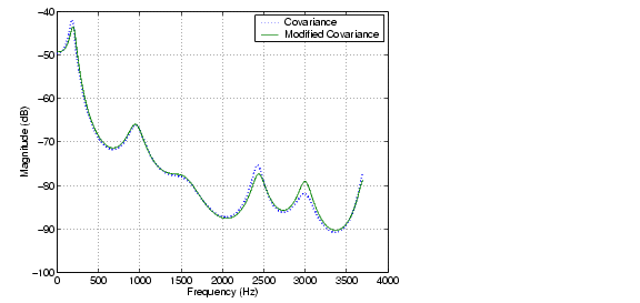
Compare the spectrum of the speech signal generated by both the covariance method and the modified covariance method. They are nearly identical, even for a short signal length:

• load mtlb
  [P1,f] = pcov(mtlb(1:64),14,1024,fs);% 14th order model
  [P2,f] = pmcov(mtlb(1:64),14,1024,fs);% 14th order model
  plot(f,10*log10(P1),':',f,10*log10(P2)); grid
  ylabel('Magnitude (dB)'); xlabel('Frequency (Hz)');
  legend('Covariance','Modified Covariance')
  
  
  

MUSIC and Eigenvector Analysis Methods

The pmusic and peig functions provide two related spectral analysis methods:

• pmusic provides the multiple signal classification (MUSIC) method developed by Schmidt
• peig provides the eigenvector (EV) method developed by Johnson

See Marple [3] (pgs. 373-378) for a summary of these methods.

Both of these methods are frequency estimator techniques based on eigenanalysis of the autocorrelation matrix. This type of spectral analysis categorizes the information in a correlation or data matrix, assigning information to either a signal subspace or a noise subspace.

Eigenanalysis Overview

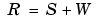
Consider a number of complex sinusoids embedded in white noise. You can write the autocorrelation matrix R for this system as the sum of the signal autocorrelation matrix (S) and the noise autocorrelation matrix (W):

There is a close relationship between the eigenvectors of the signal autocorrelation matrix and the signal and noise subspaces. The eigenvectors v of S span the same signal subspace as the signal vectors. If the system contains M complex sinusoids and the order of the autocorrelation matrix is p, eigenvectors v_M+1 through v_p+1 span the noise subspace of the autocorrelation matrix.

Frequency Estimator Functions.   To generate their frequency estimates, eigenanalysis methods calculate functions of the vectors in the signal and noise subspaces. Both the MUSIC and EV techniques choose a function that goes to infinity (denominator goes to zero) at one of the sinusoidal frequencies in the input signal. Using digital technology, the resulting estimate has sharp peaks at the frequencies of interest; this means that there might not be infinity values in the vectors.

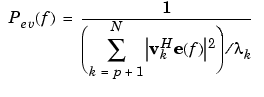
The MUSIC estimate is given by the formula

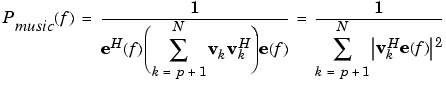
where N is the size of the eigenvectors and e(f) is a vector of complex sinusoids.

v represents the eigenvectors of the input signal's correlation matrix; v_k is the k^th eigenvector. H is the conjugate transpose operator. The eigenvectors used in the sum correspond to the smallest eigenvalues and span the noise subspace (p is the size of the signal subspace).

The expression is equivalent to a Fourier transform (the vector e(f) consists of complex exponentials). This form is useful for numeric computation because the FFT can be computed for each v_k and then the squared magnitudes can be summed.

The EV method weights the summation by the eigenvalues of the correlation matrix:

The pmusic and peig functions in this toolbox use the svd (singular value decomposition) function in the signal case and the eig function for analyzing the correlation matrix and assigning eigenvectors to the signal or noise subspaces. When svd is used, pmusic and peig never compute the correlation matrix explicitly, but the singular values are the eigenvalues.

Performance of the Periodogram

Selected Bibliography