
| Optimization Toolbox |   |
Main Algorithm
The algorithm begins by applying a series of preprocessing steps (see Preprocessing). After preprocessing, the problem has the form

|
(4-15) |
The upper bounds constraints are implicitly included in the constraint matrix A. With the addition of primal slack variables s, Eq. 4-15 becomes

|
(4-16) |
which is referred to as the primal problem: x consists of the primal variables and s consists of the primal slack variables. The dual problem is

|
(4-17) |
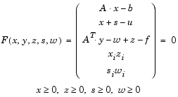
where y and w consist of the dual variables and z consists of the dual slacks. The optimality conditions for this linear program, i.e., the primal Eq. 4-16 and the dual Eq. 4-17, are

|
(4-18) |
where  and
and  denote component-wise multiplication.
The quadratic equations  and
and  are called the complementarity conditions for the linear program; the other (linear) equations are called the feasibility conditions. The quantity

is the duality gap, which measures the residual of the complementarity portion of F when  .
.
The algorithm is a primal-dual algorithm, meaning that both the primal and the dual programs are solved simultaneously. It can be considered a Newton-like method, applied to the linear-quadratic system  in Eq. 4-18, while at the same time keeping the iterates x, z, w, and s positive, thus the name interior-point method. (The iterates are in the strictly interior region represented by the inequality constraints in Eq. 4-16.)
The algorithm is a variant of the predictor-corrector algorithm proposed by Mehrotra. Consider an iterate  , where
 First compute the so-called prediction direction

which is the Newton direction; then the so-called corrector direction

where  is called the centering parameter and must be chosen carefully.
  is a zero-one vector with the ones corresponding to the quadratic equations in F(v), i.e., the perturbations are only applied to the complementarity conditions, which are all quadratic, but not to the feasibility conditions, which are all linear. The two directions are combined with a step-length parameter
  and update v to obtain the new iterate

where the step-length parameter  is chosen so that


In solving for the preceding steps, the algorithm computes a (sparse) direct factorization on a modification of the Cholesky factors of  If A has dense columns, it instead uses the Sherman-Morrison formula, and if that solution is not adequate (the residual is too large), it uses preconditioned conjugate gradients to find a solution.
The algorithm then repeats these steps until the iterates converge. The main stopping criteria is a standard one


are the primal residual, dual residual, and upper-bound feasibility respectively, and

is the difference between the primal and dual objective values, and tol is some tolerance. The sum in the stopping criteria measures the total relative errors in the optimality conditions in Eq. 4-18.
 | Large-Scale Linear Programming | Preprocessing |  |