cp2tform (Image Processing Toolbox)

Infer geometric transformation from control point pairs

Syntax

TFORM = cp2tform(input_points,base_points,transformtype)
TFORM = cp2tform(CPSTRUCT,transformtype)
TFORM = cp2tform(input_points,base_points,transformtype,parameter)
TFORM = cp2tform(CPSTRUCT,transformtype,parameter)
[TFORM,input_points,base_points] = cp2tform(CPSTRUCT,...)
[TFORM,input_points,base_points,input_points_bad,base_points_bad] 
= cp2tform(...,'piecewise linear')

Description

TFORM = cp2tform(input_points,base_points,transformtype) takes pairs of control points and uses them to infer a spatial transformation. The function returns a TFORM structure containing the spatial transformation. input_points is an m-by-2 double matrix containing the x and y coordinates of control points in the image you want to transform. base_points is an m-by-2 double matrix containing the x and y coordinates of control points specified in the base image. The transformtype argument specifies the type of transformation you want to infer. For more information about supported types, see Transform Type.

TFORM = cp2tform(CPSTRUCT,transformtype) passes a CPSTRUCT structure that contains the control point matrices for the input and base images. The Control Point Selection Tool, cpselect, creates the CPSTRUCT.

[TFORM,input_points,base_points] = cp2tform(CPSTRUCT,...) returns the control points that were actually used in input_points, and base_points. Unmatched and predicted points are not used. For more information, see cpstruct2pairs.

Transform Type

transformtype specifies the type of spatial transformation to infer. This table lists all of the transformation types supported by cp2tform, in order of complexity. (See Algorithms for detailed information about each transform type.) The table includes the minimum number of control point pairs you must select for each type. The 'lwm' and 'polynomial' transform types can each take an optional, additional parameter. See the syntax descriptions that follow for details.

Transformation Type
Description
Minimum Control Points
Example

'linear conformal'
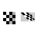
Use this transformation when shapes in the input image are unchanged, but the image is distorted by some combination of translation, rotation, and scaling. Straight lines remain straight, and parallel lines are still parallel.
2 pairs

'affine'
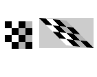
Use this transformation when shapes in the input image exhibit shearing. Straight lines remain straight, and parallel lines remain parallel, but rectangles become parallelograms.
3 pairs

'projective'
Use this transformation when the scene appears "tilted." Straight lines remain straight, but parallel lines converge toward "vanishing points" which may or may not fall within the image.
4 pairs

'polynomial'
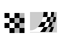
Use this transformation when objects in the image are curved. The higher the order of the polynomial, the better the fit, but the result can contain more curves than the base image.
6 pairs
(order 2)
10 pairs
(order 3)
16 pairs
(order 4)

'piecewise linear'
Use this transformation when parts of the image appear distorted differently.
4 pairs

'lwm'
Use this transformation (local weighted mean), when the distortion varies locally and piecewise linear is not sufficient.
6 pairs
(12 pairs recommended)

Transformation Type	Description	Minimum Control Points	Example
'linear conformal'	Use this transformation when shapes in the input image are unchanged, but the image is distorted by some combination of translation, rotation, and scaling. Straight lines remain straight, and parallel lines are still parallel.	2 pairs
'affine'	Use this transformation when shapes in the input image exhibit shearing. Straight lines remain straight, and parallel lines remain parallel, but rectangles become parallelograms.	3 pairs
'projective'	Use this transformation when the scene appears "tilted." Straight lines remain straight, but parallel lines converge toward "vanishing points" which may or may not fall within the image.	4 pairs
'polynomial'	Use this transformation when objects in the image are curved. The higher the order of the polynomial, the better the fit, but the result can contain more curves than the base image.	6 pairs (order 2) 10 pairs (order 3) 16 pairs (order 4)
'piecewise linear'	Use this transformation when parts of the image appear distorted differently.	4 pairs
'lwm'	Use this transformation (local weighted mean), when the distortion varies locally and piecewise linear is not sufficient.	6 pairs (12 pairs recommended)

Note When transformtype is 'linear conformal', 'affine', 'projective', or 'polynomial', and input_points and base_points (or CPSTRUCT) have the minimum number of control points needed for a particular transformation, cp2tform finds the coefficients exactly. If input_points and base_points include more than the minimum number of points, cp2tform uses a least squares solution. For more information, see mldivide.

TFORM = cp2tform(input_points,base_points,'polynomial',ORDER) TFORM = cp2tform(CPSTRUCT,'polynomial',order)

When 'polynomial' is the transform type, you can optionally specify the order of the polynomial to use. order can be the scalar value 2, 3, or 4. If you omit order, it defaults to 3.

TFORM = cp2tform(input_points,base_points,'lwm',N) TFORM = cp2tform(CPSTRUCT,'lwm',N)

When 'lwm' is the transform type, you can optionally specify the number of points, N, used to infer each polynomial. The radius of influence extends out to the furthest control point used to infer that polynomial. The N closest points are used to infer a polynomial of order 2 for each control point pair. If you omit N, it defaults to 12. N can be as small as 6, but making N small risks generating ill-conditioned polynomials.

[TFORM,input_points,base_points,input_points_bad,base_points_bad]= cp2tform(input_points,base_points,'piecewise linear') [TFORM,input_points,base_points,input_points_bad,base_points_bad]= cp2tform(CPSTRUCT,'piecewise linear')

When 'piecewise linear' is the transform type, cp2tform can optionally return the control points that were actually used in input_points and base_points, and return two arrays, input_points_bad and base_points_bad, that contain control points that were eliminated because they were middle vertices of degenerate fold-over triangles.

Algorithms

cp2tform uses the following general procedure:

Use valid pairs of control points to infer a spatial transformation or an inverse-mapping from output space (x,y) to input space (u,v) according to transformtype.
Return TFORM structure containing spatial transformation.

The procedure varies depending on the transformtype.

Linear Conformal

Linear conformal transformations may include a rotation, a scaling, and a translation. Shapes and angles are preserved. Parallel lines remain parallel. Straight lines remain straight.

Let:

sc = scale*cos(angle)
ss = scale*sin(angle)

[u v] = [x y 1] * [ sc -ss
                    ss  sc
                    tx  ty]

Solve for sc, ss, tx, ty.

t_lc = cp2tform(input_points,base_points,'linear conformal');

The coefficients of the inverse mapping are stored in t_lc.tdata.Tinv.

Since linear conformal transformations are a subset of affine transformations, t_lc.forward_fcn is @affine_fwd and t_lc.inverse_fcn is @affine_inv.

At least two control-point pairs are needed to solve for the four unknown coefficients.

Affine

In an affine transformation, the x and y dimensions can be scaled or sheared independently and there may be a translation. Parallel lines remain parallel. Straight lines remain straight. Linear conformal transformations are a subset of affine transformations.

For an affine transformation:

```
[u v] = [x y 1] * Tinv 
```

Tinv is a 3-by-2 matrix. Solve for the 6 elements of Tinv.

t_affine = cp2tform(input_points,base_points,'affine');

The coefficients of the inverse mapping are stored in t_affine.tdata.Tinv.

At least 3 control-point pairs are needed to solve for the 6 unknown coefficients.

Projective

In a projective transformation, quadrilaterals map to quadrilaterals. Straight lines remain straight. Affine transformations are a subset of projective transformations.

For a projective transformation:

```
[up vp wp] = [x y w] * Tinv
```

where

```
u = up/wp 
v = vp/wp
```

Tinv is a 3-by-3 matrix.

Assuming

Tinv = [ A D G;
         B E H;
         C F I ];
u = (Ax + By + C)/(Gx + Hy + I)
v = (Dx + Ey + F)/(Gx + Hy + I)

Solve for the 9 elements of Tinv.

t_proj = cp2tform(input_points,base_points,'projective');

The coefficients of the inverse mapping are stored in t_proj.tdata.Tinv.

At least 4 control-point pairs are needed to solve for the 9 unknown coefficients.

Polynomial

In a polynomial transformation, polynomial functions of x and y determine the mapping.

Second-Order Polynomials

For a second-order polynomial transformation:

[u v] = [1 x y x*y x^2 y^2] * Tinv

Both u and v are second-order polynomials of x and y. Each second-order polynomial has six terms. To specify all coefficients, Tinv has size 6-by-2.

t_poly_ord2 = cp2tform(input_points,base_points,'polynomial');

The coefficients of the inverse mapping are stored in t_poly_ord2.tdata.

At least 6 control-point pairs are needed to solve for the 12 unknown coefficients.

Second-Order Polynomials
For a second-order polynomial transformation: [u v] = [1 x y xy x^2 y^2] Tinv Both `u` and `v` are second-order polynomials of `x` and `y`. Each second-order polynomial has six terms. To specify all coefficients, `Tinv` has size 6-by-2. t_poly_ord2 = cp2tform(input_points,base_points,'polynomial'); The coefficients of the inverse mapping are stored in `t_poly_ord2.tdata`. At least 6 control-point pairs are needed to solve for the 12 unknown coefficients.

Third-Order Polynomials

For a third-order polynomial transformation:

[u v] = [1 x y x*y x^2 y^2 y*x^2 x*y^2 x^3 y^3] * Tinv

Both u and v are third-order polynomials of x and y. Each third-order polynomial has ten terms. To specify all coefficients, Tinv has size 10-by-2.

t_poly_ord3 = cp2tform(input_points, base_points, 'polynomial',3);

The coefficients of the inverse mapping are stored in t_poly_ord3.tdata.

At least 10 control-point pairs are needed to solve for the 20 unknown coefficients.

Third-Order Polynomials
For a third-order polynomial transformation: [u v] = [1 x y xy x^2 y^2 yx^2 xy^2 x^3 y^3] Tinv Both `u` and `v` are third-order polynomials of `x` and `y`. Each third-order polynomial has ten terms. To specify all coefficients, `Tinv` has size 10-by-2. t_poly_ord3 = cp2tform(input_points, base_points, 'polynomial',3); The coefficients of the inverse mapping are stored in `t_poly_ord3.tdata`. At least 10 control-point pairs are needed to solve for the 20 unknown coefficients.

Fourth-Order Polynomials

For a fourth-order polynomial transformation:

[u v] = [1 x y x*y x^2 y^2 y*x^2 x*y^2 x^3 y^3] * Tinv

Both u and v are fourth-order polynomials of x and y. Each fourth-order polynomial has fifteen terms. To specify all coefficients, Tinv has size 15-by-2.

t_poly_ord4 = cp2tform(input_points, base_points, 'polynomial',4);

The coefficients of the inverse mapping are stored in t_poly_ord4.tdata.

At least 15 control-point pairs are needed to solve for the 30 unknown coefficients.

Fourth-Order Polynomials
For a fourth-order polynomial transformation: [u v] = [1 x y xy x^2 y^2 yx^2 xy^2 x^3 y^3] Tinv Both `u` and `v` are fourth-order polynomials of `x` and `y`. Each fourth-order polynomial has fifteen terms. To specify all coefficients, `Tinv` has size 15-by-2. t_poly_ord4 = cp2tform(input_points, base_points, 'polynomial',4); The coefficients of the inverse mapping are stored in `t_poly_ord4.tdata`. At least 15 control-point pairs are needed to solve for the 30 unknown coefficients.

Piecewise Linear

In a piecewise linear transformation, linear (affine) transformations are applied separately to each triangular region of the image [1].

Find a Delaunay triangulation of the base control points.
Using the 3 vertices of each triangle, infer an affine mapping from base to input coordinates.

Note At least 4 control-point pairs are needed. Four pairs result in two triangles with distinct mappings.

Local Weighted Mean

For each control point in base_points:

Find the N closest control points.
Use these N points and their corresponding points in input_points to infer a second order polynomial.
Calculate the radius of influence of this polynomial as the distance from the center control point to the furthest point used to infer the polynomial (using base_points). [2]

Note At least 6 control-point pairs are needed to solve for the second-order polynomial. Ill-conditioned polynomials may result if too few pairs are used.

Example

I = checkerboard;
J = imrotate(I,30);
base_points = [11 11; 41 71];
input_points = [14 44; 70 81];
cpselect(J,I,input_points,base_points);

t = cp2tform(input_points,base_points,'linear conformal');

To recover angle and scale:

ss = t.tdata.Tinv(2,1); % ss = scale * sin(angle)
sc = t.tdata.Tinv(1,1); % sc = scale * cos(angle)
angle = atan2(ss,sc)*180/pi
scale = sqrt(ss*ss + sc*sc)

References

[1] Ardeshir Goshtasby, Piecewise linear mapping functions for image registration, Pattern Recognition, Vol 19, pp. 459-466, 1986.

[2] Ardeshir Goshtasby, Image registration by local approximation methods, Image and Vision Computing, Vol 6, p. 255-261, 1988.

corr2 cpcorr