System Identification Toolbox

Multivariable ARX Models: The idarx Model

A multivariable ARX model with nu inputs and ny outputs is given by

(3-45)

Here A(q) is an ny-by-ny matrix whose entries are polynomials in the delay operator q^-1. You can represent it as

(3-46)

as well as the matrix

(3-47)

where the entries are polynomials in the delay operator :

(3-48)

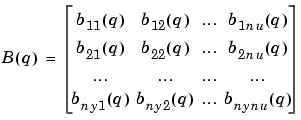
This polynomial describes how old values of output number j affect output number k. Here is the Kronecker-delta; it equals 1 when , otherwise, it is 0. Similarly, is an ny-by-nu matrix

(3-49)

or

(3-50)

with

The delay from input number j to output number k is . To link with the structure definition in terms of na, nb, nk in the arx and iv4 commands, note that na is a matrix whose kj-element is , while the kj-elements of nb and nk are and respectively.

The idarx representation of the model (3-45) can be created by

• m = idarx(A,B)
  

where A and B are 3-D arrays of dimensions ny-by-ny-by-(na+1) and ny-by-nu-by-(nb+1), respectively, that define the matrix polynomials (3-46) and (3-49).

• A(:,:,k+1) = Ak 
  B(:,:,k+1) = Bk 
  

Note that A(:,:,1) is always the identity matrix, and that leading zero coefficients in B matrices define the delays.

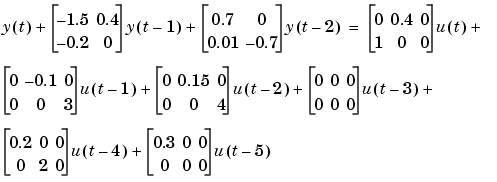
Consider the following system with two outputs and three inputs.

which in matrix notation can be written as

This system is defined and simulated for a certain input u, and then estimated in the correct ARX structure by the following string of commands.

• A(:,:,1) = eye(2);
  A(:,:,2) = [-1.5 0.4; -0.2 0];
  A(:,:,3) = [0.7 0 ; 0.01 -0.7];
  B(:,:,1) = [0 0.4 0;1 0 0];
  B(:,:,2) = [0 -0.1 0;0 0 3];
  B(:,:,3) = [0 0.15 0;0 0 4];
  B(:,:,4) = [0 0 0;0 0 0];
  B(:,:,5) = [0.2 0 0;0 2 0];
  B(:,:,6) = [0.3 0 0;0 0 0];
  m0 = idarx(A,B);
  u = iddata([], idinput([200,3]));
  e = iddata([], randn(200,2));
  y = sim(m0, [u e]);
  na = [2 1;2 2];
  nb = [2 3 0;1 1 2];
  nk = [4 0 0;0 4 1];
  me = arx([y u],[na nb nk])
  me.a % The estimated A-polynominal
  

Polynomial Black-Box Models: The idpoly Model

Black-Box State-Space Models: the idss Model