Getting Started with the Blockset (Fixed-Point Blockset)

Fixed-Point Blockset

Configuring Fixed-Point Blocks

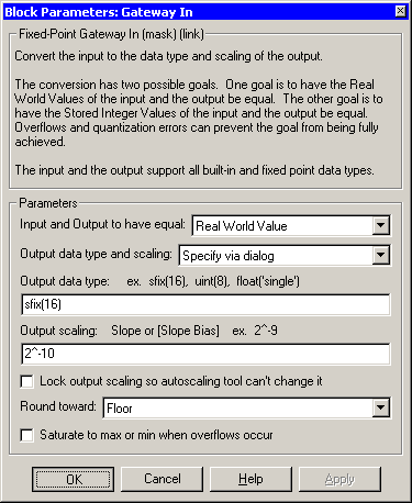
You configure fixed-point blocks with a parameter dialog box. To configure blocks, you supply values for parameters via editable text fields, check boxes, and parameter lists. The dialog box for the Gateway In block is shown below.

The following sections discuss parameters associated with this block.

For detailed information about each fixed-point block, refer to Block Reference.

Real-World Values Versus Integer Values

You can configure the fixed-point gateway blocks to treat signals as real-world values or as stored integers with the Input and output to have equal parameter. The possible values are Real World Value and Stored Integer.

In terms of the variables defined in The General [Slope Bias] Encoding Scheme, the real-world value is given by V and the stored integer value is given by Q. You may want to treat numbers as stored integer values if you are modeling hardware that produces integers as output.

Selecting the Output Data Type

For many fixed-point blocks, you have the option of specifying the output data type via the block dialog box, or inheriting the output data type from another block. You control how the output data type is selected with the Output data type and scaling or Output data type mode parameter list. Some possible values are Specify via dialog, Inherit via internal rule, Inherit via back propagation and Same as input.

The Fixed-Point Blockset supports several fixed-point and floating-point data types. Fixed-point data types are characterized by their word size in bits and by their radix (binary) point. The radix point is the means by which fixed-point values are scaled. Additionally

Unsigned and two's complement formats are supported.
The fixed-point word size can range from 1 to 128 bits in simulation.
The radix point is not required to be contiguous with the fixed-point word.

Floating-point data types are characterized by their sign bit, fraction (mantissa) field, and exponent field. The Fixed-Point Blockset supports IEEE singles, IEEE doubles, and a nonstandard IEEE-style floating-point data type.

Note You can create Fixed-Point Blockset data types directly in the MATLAB workspace and then pass the resulting structure to a fixed-point block, or you can specify the data type directly with the block dialog box.

Integers. You specify unsigned and signed integers with the uint and sint functions, respectively.

For example, to specify a 16-bit unsigned integer via the block dialog box, you configure the Output data type parameter as uint(16). To specify a 16-bit signed integer, you configure the Output data type parameter as sint(16).

For integer data types, the default radix point is assumed to lie to the right of all bits.

Fractional Numbers. You specify unsigned and signed fractional numbers with the ufrac and sfrac functions, respectively.

For example, to configure the output as a 16-bit unsigned fractional number via the block dialog box, you specify the Output data type parameter to be ufrac(16). To configure a 16-bit signed fractional number, you specify Output data type to be sfrac(16).

Fractional numbers are distinguished from integers by their default scaling. Whereas signed and unsigned integer data types have a default radix point to the right of all bits, unsigned fractional data types have a default radix point to the left of all bits, while signed fractional data types have a default radix point to the right of the sign bit.

Both unsigned and signed fractional data types support guard bits, which act to "guard" against overflow. For example, sfrac(16,4) specifies a 16-bit signed fractional number with 4 guard bits. The guard bits lie to the left of the default radix point.

Generalized Fixed-Point Numbers. You specify unsigned and signed generalized fixed-point numbers with the ufix and sfix functions. respectively.

For example, to configure the output as a 16-bit unsigned generalized fixed-point number via the block dialog box, you specify the Output data type parameter to be ufix(16). To configure a 16-bit signed generalized fixed-point number, you specify Output data type to be sfix(16).

Generalized fixed-point numbers are distinguished from integers and fractionals by the absence of a default scaling. For these data types, you must explicitly specify the scaling with the Output scaling or Output scaling value parameter, or inherit the scaling from another block. Refer to Selecting the Output Scaling for more information.

Floating-Point Numbers. The Fixed-Point Blockset supports single-precision and double-precision floating-point numbers as defined by the IEEE Standard 754-1985 for Binary Floating-Point Arithmetic. You specify floating-point numbers with the float function.

For example, to configure the output as a single-precision floating-point number via the block dialog box, you specify the Output data type parameter to be float('single'). To configure a double-precision floating-point number, you specify Output data type to be float('double').

You can also specify a nonstandard floating-point number that mimics the IEEE style. For this data type, the fraction (mantissa) can range from 1 to 52 bits and the exponent can range from 1 to 11 bits. For example, to configure a nonstandard floating-point number having 32 total bits and 9 exponents bits, you specify Output data type to be float(32,9).

Note These numbers are normalized with a hidden leading 1 for all exponents except the smallest possible exponent. However, the largest possible exponent might not be treated as a flag for Infs or NaNs.

Selecting the Output Scaling

Most data types supported by the Fixed-Point Blockset have a default scaling that you cannot change. However, for generalized fixed-point data types, you have the option of specifying the output scaling via the block dialog box, or inheriting the output scaling from another block. You control how the output scaling is selected with the Output data type and scaling or Output data type mode parameter.

The Fixed-Point Blockset supports two general scaling modes: radix point-only scaling and [Slope Bias] scaling. In addition to these general scaling modes, the blockset provides you with additional block-specific scaling choices for constant vectors and constant matrices. These scaling choices are based on radix point-only scaling and are designed to maximize precision. Refer to Example: Constant Scaling for Best Precision for more information.

To help you understand the supported scaling modes, the general [Slope Bias] encoding scheme is presented in the next section.

The General [Slope Bias] Encoding Scheme. When representing an arbitrarily precise real-world value with a fixed-point number, it is often useful to define a general [Slope Bias] encoding scheme

where

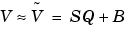
is the real-world value.
is the approximate real-world value.
Q is an integer that encodes V.
B is the bias.
S = F2^Eis the slope.

The slope is partitioned into two components:

2^Especifies the radix point. E is the fixed power-of-two exponent.
F is the fractional slope. It is normalized such that .

Radix Point-Only Scaling. This is "powers-of-two" scaling since it involves moving only the radix point. Radix point-only scaling does not require the radix point to be contiguous with the data word. The advantage of this scaling mode is the number of processor arithmetic operations is minimized.

You specify radix point-only scaling with the syntax 2^-E where E is unrestricted. This creates a MATLAB structure with a bias B = 0 and a fractional slope F = 1.0.

For example, if you specify the value 2^-10 for the Output scaling or Output scaling value parameter, then the generalized fixed-point number has a power-of-two exponent E = -10. This value defines the radix point location to be 10 places to the left of the least significant bit.

[Slope Bias] Scaling. With this scaling mode, you can provide a slope and a bias. The advantage of [Slope Bias] scaling is that it typically provides more efficient use of a finite number of bits.

You specify [Slope Bias] scaling with the syntax [slope bias], which creates a MATLAB structure with the given slope and bias.

For example, if you specify the value [5/9 10] for the Output scaling or Output scaling value parameter, then the generalized fixed-point number has a slope of 5/9 and a bias of 10. The blockset would automatically store F as 1.1111 and E as -1 due to the normalization condition .

Rounding

You specify how fixed-point numbers are rounded with the Round toward or Round integer calculations toward parameter. These rounding modes are supported:

Zero - This mode rounds toward zero and is equivalent to the MATLAB fix function.
Nearest - This mode rounds toward the nearest representable number, with the exact midpoint rounded toward positive infinity. Rounding toward nearest is equivalent to the MATLAB round function.
Ceiling - This mode rounds toward positive infinity and is equivalent to the MATLAB ceil function.
Floor - This mode rounds toward negative infinity and is equivalent to the MATLAB floor function.

Overflow Handling

You control how overflow conditions are handled for fixed-point operations with the Saturate to max or min when overflows occur or Saturate on integer overflow checkbox.

If this box is selected, then overflows saturate to either the maximum or minimum value represented by the data type. For example, an overflow associated with a signed 8-bit integer can saturate to -128 or 127.

If this box is not selected, then overflows wrap to the appropriate value that is representable by the data type. For example, the number 130 does not fit in a signed 8-bit integer, and would wrap to -126.

Locking the Output Scaling

If the output data type is a generalized fixed-point number, then you have the option of locking its scaling by checking the Lock output scaling so autoscaling tool can't change it or Lock output scaling against changes by the autoscaling tool checkbox.

When locked, the automatic scaling script autofixexp will not change the output scaling. Otherwise, the autofixexp is free to adjust the scaling.

Overview of Blockset Features Additional Features and Capabilities