Financial Toolbox

Plotting Sensitivities of a Portfolio of Options

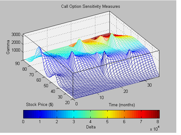
This example plots gamma as a function of price and time for a portfolio of 10 Black-Scholes options. The plot shows a three-dimensional surface. For each point on the surface, the height (z-value) represents the sum of the gammas for each option in the portfolio weighted by the amount of each option. The x-axis represents changing price, and the y-axis represents time. The plot adds a fourth dimension by showing delta as surface color. This example M-file is ftgex3.m.

First set up the portfolio with arbitrary data. Current prices range from $20 to $90 for each option. Set corresponding exercise prices for each option.

• Range = 20:90;
  PLen = length(Range);
  ExPrice = [75 70 50 55 75 50 40 75 60 35];
  

Set all risk-free interest rates to 10%, and set times to maturity in days. Set all volatilities to 0.35. Set the number of options of each instrument, and allocate space for matrices.

• Rate = 0.1*ones(10,1);
  Time = [36  36  36  27  18  18  18  9  9  9];
  Sigma = 0.35*ones(10,1);
  NumOpt = 1000*[4  8  3  5  5.5  2  4.8  3  4.8  2.5];
  ZVal = zeros(36, PLen);
  Color = zeros(36, PLen);
  

For each instrument, create a matrix (of size Time by PLen) of prices for each period.

• for i = 1:10
      Pad = ones(Time(i),PLen);
      NewR = Range(ones(Time(i),1),:);
  

Create a vector of time periods 1 to Time; and a matrix of times, one column for each price.

•     T = (1:Time(i))';
      NewT = T(:,ones(PLen,1));
  

Call the toolbox gamma and delta sensitivity functions to compute gamma and delta.

•     ZVal(36-Time(i)+1:36,:) = ZVal(36-Time(i)+1:36,:) ...
          + NumOpt(i) * blsgamma(NewR, ExPrice(i)*Pad, ...
          Rate(i)*Pad, NewT/36, Sigma(i)*Pad);
  
      Color(36-Time(i)+1:36,:) = Color(36-Time(i)+1:36,:) ...
          + NumOpt(i) * blsdelta(NewR, ExPrice(i)*Pad, ...
          Rate(i)*Pad, NewT/36, Sigma(i)*Pad);
  end
  

Draw the surface as a mesh, set the viewpoint, and reverse the x-axis because of the viewpoint. The axes range from 20 to 90, 0 to 36, and - to .

• mesh(Range, 1:36, ZVal, Color);
  view(60,60);
  set(gca, 'xdir','reverse');
  axis([20 90  0 36  -inf inf]);
  

Add a title and axis labels and draw a box around the plot. Annotate the colors with a bar and label the colorbar.

• title('Call Option Sensitivity Measures');
  xlabel('Stock Price ($)');
  ylabel('Time (months)');
  zlabel('Gamma');
  set(gca, 'box', 'on');
  colorbar('horiz');
  a = findobj(gcf, 'type', 'axes');
  set(get(a(2), 'xlabel'), 'string', 'Delta');
  
  
  

Plotting Sensitivities of an Option

Function Reference