Getting Started

Plotting and Comparing Multiple Systems

You can use the command-line response-plotting functions to plot the response of continuous and discrete linear models on a single plot. To do so, invoke the corresponding command-line function using the list sys1,..., sysN of models as the inputs.

• step(sys1,sys2,...,sysN)
  impulse(sys1,sys2,...,sysN)
  ...
  bode(sys1,sys2,...,sysN)
  nichols(sys1,sys2,...,sysN)
  ...
  

All models in the argument lists of any of the response plotting functions (except for sigma) must have the same number of inputs and outputs. To differentiate the plots easily, you can also specify a distinctive color/linestyle/marker for each system just as you would with the plot command. For example,

• bode(sys1,'r',sys2,'y--',sys3,'gx')
  

plots sys1 with solid red lines, sys2 with yellow dashed lines, and sys3 with green x markers.

You can plot responses of multiple models on the same plot. These models do not need to be all continuous-time or all discrete-time.

Example: Comparing Continuous and Discretized Systems

The following example compares a continuous model with its zero-order-hold discretization.

• sysc = tf(1000,[1 10 1000])
  sysd = c2d(sysc,0.2)        % ZOH sampled at 0.2 second
  
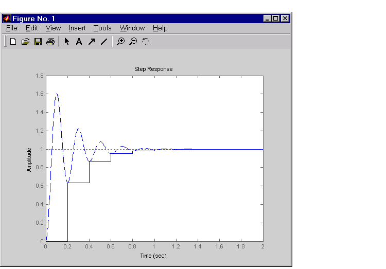
  step(sysc,'--',sysd,'-')    % Compare step responses
  

These commands produce the plot shown below.

Figure 3-16: Comparison of a Continuous Model to Its Discretized Version

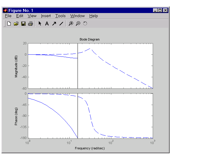
Use this command to compare the Bode plots of the two systems.

• bode(sysc,'--',sysd,'-')     % Compare Bode responses
  

The Control System Toolbox creates this plot.

Figure 3-17: Comparison of Bode Plots for a Continuous Model and Its Discretized Version

A comparison of the continuous and discretized responses reveals a drastic undersampling of the continuous-time system. Specifically, there are hidden oscillations in the discretized time response and aliasing conceals the continuous-time resonance near 30 rad/sec.

Data Markers

Creating Custom Plots