| Mathematics | |
Example: Electrodynamics Problem
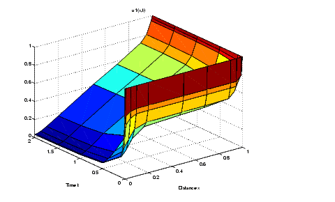
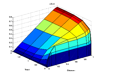
This example illustrates the solution of a system of partial differential equations. The problem is taken from electrodynamics. It has boundary layers at both ends of the interval, and the solution changes rapidly for small  .
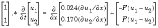
.
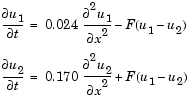
where
 . The equations hold on an interval
  for times
  .
.
The solution  satisfies the initial conditions

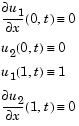
Note
The demo pdex4 contains the complete code for this example. The demo uses subfunctions to place all required functions in a single M-file. To run this example type pdex4 at the command line. See PDE Solver Basic Syntax and Solving PDE Problems for more information.
|
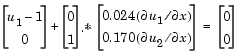
 have to be written in terms of the flux. In the form expected by
 pdepe, the left boundary condition is
and the right boundary condition is
pdepe can use. The function must be of the form
c, f, and s correspond to the  ,
,  , and
, and  terms in Equation 14-4.
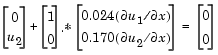
 and
and  (Equation 14-6) of the boundary conditions in the function
 pdex4bc.
 . The program selects the step size in time to resolve this sharp change, but to see this behavior in the plots, output times must be selected accordingly. There are boundary layers in the solution at both ends of [0,1], so mesh points must be placed there to resolve these sharp changes. Often some experimentation is needed to select the mesh that reveals the behavior of the solution.
x = [0 0.005 0.01 0.05 0.1 0.2 0.5 0.7 0.9 0.95 0.99 0.995 1];
t = [0 0.005 0.01 0.05 0.1 0.5 1 1.5 2];
pdepe with m = 0, the functions pdex4pde, pdex4ic, and pdex4bc, and the mesh defined by x and t at which pdepe is to evaluate the solution. The pdepe function returns the numerical solution in a three-dimensional array sol, where sol(i,j,k) approximates the kth component of the solution,  , evaluated at
 t(i) and x(j).
| | Changing PDE Integration Properties | Selected Bibliography | |