Optimization Toolbox

Introduction

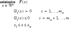
Multiobjective optimization is concerned with the minimization of a vector of objectives F(x) that can be the subject of a number of constraints or bounds.

(3-47)

Note that, because F(x) is a vector, if any of the components of F(x) are competing, there is no unique solution to this problem. Instead, the concept of noninferiority [41] (also called Pareto optimality [4],[6]) must be used to characterize the objectives. A noninferior solution is one in which an improvement in one objective requires a degradation of another. To define this concept more precisely, consider a feasible region, , in the parameter space that satisfies all the constraints, i.e.,

(3-48)

subject to

This allows us to define the corresponding feasible region for the objective function space .

where subject to

(3-49)

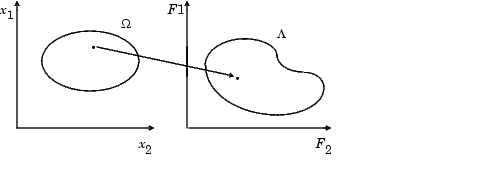
The performance vector, F(x), maps parameter space into objective function space as is represented for a two-dimensional case in Figure 3-7.

Figure 3-7: Mapping from Parameter Space into Objective Function Space

A noninferior solution point can now be defined.

Definition: A point is a noninferior solution if for some neighborhood of there does not exist a such that and

(3-50)

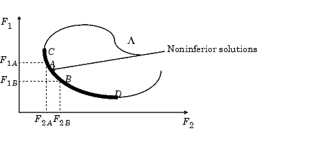
In the two-dimensional representation of Figure 3-8, Set of Noninferior Solutions, the set of noninferior solutions lies on the curve between C and D. Points A and B represent specific noninferior points.

Figure 3-8: Set of Noninferior Solutions

A and B are clearly noninferior solution points because an improvement in one objective, , requires a degradation in the other objective, , i.e.,

.

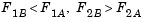Since any point in that is not a noninferior point represents a point in which improvement can be attained in all the objectives, it is clear that such a point is of no value. Multiobjective optimization is, therefore, concerned with the generation and selection of noninferior solution points. The techniques for multiobjective optimization are wide and varied and all the methods cannot be covered within the scope of this toolbox. Subsequent sections describe some of the techniques.

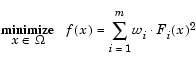
Weighted Sum Strategy

The weighted sum strategy converts the multiobjective problem of minimizing the vector into a scalar problem by constructing a weighted sum of all the objectives.

(3-51)

The problem can then be optimized using a standard unconstrained optimization algorithm. The problem here is in attaching weighting coefficients to each of the objectives. The weighting coefficients do not necessarily correspond directly to the relative importance of the objectives or allow tradeoffs between the objectives to be expressed. Further, the noninferior solution boundary can be nonconcurrent, so that certain solutions are not accessible.

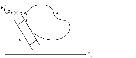
This can be illustrated geometrically. Consider the two-objective case in Figure 3-9, Geometrical Representation of the Weighted Sum Method. In the objective function space a line, L, is drawn. The minimization of Eq. 3-51 can be interpreted as finding the value of c for which L just touches the boundary of as it proceeds outwards from the origin. Selection of weights and , therefore, defines the slope of L, which in turn leads to the solution point where L touches the boundary of .

Figure 3-9: Geometrical Representation of the Weighted Sum Method

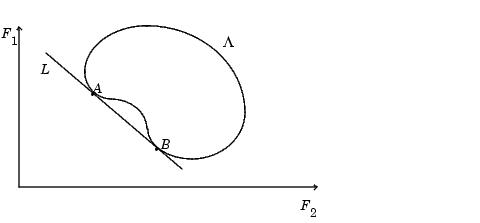
The aforementioned convexity problem arises when the lower boundary of is nonconvex as shown in Figure 3-10, Nonconvex Solution Boundary. In this case the set of noninferior solutions between A and B is not available.

Figure 3-10: Nonconvex Solution Boundary

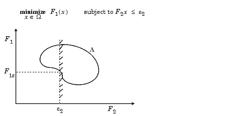
-Constraint Method

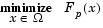
A procedure that overcomes some of the convexity problems of the weighted sum technique is the -constraint method. This involves minimizing a primary objective, , and expressing the other objectives in the form of inequality constraints

(3-52)

subject to

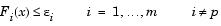
Figure 3-11, Geometrical Representation of e-Constraint Method, shows a two-dimensional representation of the -constraint method for a two-objective problem.

Figure 3-11: Geometrical Representation of -Constraint Method

This approach is able to identify a number of noninferior solutions on a nonconvex boundary that are not obtainable using the weighted sum technique, for example, at the solution point and . A problem with this method is, however, a suitable selection of to ensure a feasible solution. A further disadvantage of this approach is that the use of hard constraints is rarely adequate for expressing true design objectives. Similar methods exist, such as that of Waltz [40], that prioritize the objectives. The optimization proceeds with reference to these priorities and allowable bounds of acceptance. The difficulty here is in expressing such information at early stages of the optimization cycle.

In order for the designers' true preferences to be put into a mathematical description, the designers must express a full table of their preferences and satisfaction levels for a range of objective value combinations. A procedure must then be realized that is able to find a solution with reference to this. Such methods have been derived for discrete functions using the branches of statistics known as decision theory and game theory (for a basic introduction, see [26]). Implementation for continuous functions requires suitable discretization strategies and complex solution methods. Since it is rare for the designer to know such detailed information, this method is deemed impractical for most practical design problems. It is, however, seen as a possible area for further research.

What is required is a formulation that is simple to express, retains the designers' preferences, and is numerically tractable.

Multiobjective Optimization

Goal Attainment Method