ugarchsim (Financial Toolbox)

Simulate a univariate GARCH(P,Q) process with Gaussian innovations

Syntax

[U, H] = ugarchsim(Kappa, Alpha, Beta, NumSamples)

Arguments

Kappa
Scalar constant term of the GARCH process.

Alpha
P-by-1 vector of coefficients, where P is the number of lags of the conditional variance included in the GARCH process. Alpha can be an empty matrix, in which case P is assumed 0; when P = 0, a GARCH(0,Q) process is actually an ARCH(Q) process.

Beta
Q-by-1 vector of coefficients, where Q is the number of lags of the squared innovations included in the GARCH process.

NumSamples
Positive, scalar integer indicating the number of samples of the innovations U and conditional variance H (see below) to simulate.

`Kappa`	Scalar constant term of the GARCH process.
`Alpha`	`P`-by-1 vector of coefficients, where `P` is the number of lags of the conditional variance included in the GARCH process. `Alpha` can be an empty matrix, in which case `P` is assumed 0; when `P = 0`, a GARCH(0,Q) process is actually an ARCH(Q) process.
`Beta`	`Q`-by-1 vector of coefficients, where `Q` is the number of lags of the squared innovations included in the GARCH process.
`NumSamples`	Positive, scalar integer indicating the number of samples of the innovations `U` and conditional variance `H` (see below) to simulate.

Description

[U, H] = ugarchsim(Kappa, Alpha, Beta, NumSamples) simulates a univariate GARCH(P,Q) process with Gaussian innovations.

U is a number of samples (NUMSAMPLES)-by-1 vector of innovations (_t), representing a mean-zero, discrete-time stochastic process. The innovations time series U is designed to follow the GARCH(P,Q) process specified by the inputs Kappa, Alpha, and Beta.

H is a NUMSAMPLES-by-1 vector of the conditional variances (_t²) corresponding to the innovations vector U. Note that U and H are the same length, and form a "matching" pair of vectors. As shown in the following equation, _t² (i.e., H(t)) represents the time series inferred from the innovations time series {_t} (i.e., U).

The time-conditional variance, _t², of a GARCH(P,Q) process is modeled as

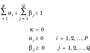
where represents the argument Alpha, represents Beta, and the GARCH(P,Q) coefficients {, , } are subject to the following constraints.

Note that U is a vector of residuals or innovations (_t) of an econometric model, representing a mean-zero, discrete-time stochastic process.

Although _t² is generated using the equation above, _t and _t² are related as

where {v_t} is an independent, identically distributed (i.i.d.) sequence ~ N(0,1).

The output vectors U and H are designed to be steady-state sequences in which transients have arbitrarily small effect. The (arbitrary) metric used by ugarchsim strips the first N samples of U and H such that the sum of the GARCH coefficients, excluding Kappa, raised to the Nth power, does not exceed 0.01.

       0.01 = (sum(Alpha) + sum(Beta))^N

Thus

       N = log(0.01)/log((sum(Alpha) + sum(Beta)))

Note ugarchsim corresponds generally to the GARCH Toolbox function garchsim. The GARCH Toolbox provides a comprehensive and integrated computing environment for the analysis of volatility in time series. For information see the GARCH Toolbox User's Guide or the financial products Web page at http://www.mathworks.com/products/finprod/.

Examples

This example simulates a GARCH(P,Q) process with P = 2 and Q = 1.

% Set the random number generator seed for reproducability.

randn('seed', 10)

% Set the simulation parameters of GARCH(P,Q) = GARCH(2,1) process.

Kappa = 0.25;      %a positive scalar.
Alpha = [0.2 0.1]'; %a column vector of nonnegative numbers (P = 2).
Beta = 0.4;        % Q = 1.
NumSamples = 500;  % number of samples to simulate.

% Now simulate the process.

[U , H] = ugarchsim(Kappa, Alpha, Beta, NumSamples);

% Estimate the process parameters.

P = 2;    % Model order P (P = length of Alpha).
Q = 1;    % Model order Q (Q = length of Beta).
[k, a, b] = ugarch(U , P , Q);
disp(' ')
disp(' Estimated Coefficients:')
disp(' -----------------------')
disp([k; a; b])
disp(' ')

% Forecast the conditional variance using the estimated   
% coefficients.

NumPeriods = 10;    % Forecast out to 10 periods.
[VarianceForecast, H1] = ugarchpred(U, k, a, b, NumPeriods);
disp(' Variance Forecasts:')
disp(' ------------------')
disp(VarianceForecast)
disp(' ')

When the above code is executed, the screen output looks like the display shown.

%%%%%%%%%%%%%%%%%%%%%%%%%%%%%%%%%%%%%%%%%%%%%%%%%%%%%%%%%%%
Diagnostic Information 

Number of variables: 4

Functions 
Objective:        ugarchllf
Gradient:         finite-differencing
Hessian:          finite-differencing (or Quasi-Newton)

Constraints
Nonlinear constraints:             do not exist
Number of linear inequality constraints:    1
Number of linear equality constraints:      0
Number of lower bound constraints:          4
Number of upper bound constraints:          0
Algorithm selected
   medium-scale

%%%%%%%%%%%%%%%%%%%%%%%%%%%%%%%%%%%%%%%%%%%%%%%%%%%%%%%%%%%
End diagnostic information 
                                       max                       Directional 
 Iter   F-count    f(x)   constraint   Step-size     derivative     Procedure 
    1     5     699.185      -0.125            1      -2.97e+006     
    2    22     658.224     -0.1249     0.000488           -64.6     
    3    28     610.181           0            1           -49.4     
    4    35     590.888           0          0.5           -38.9     
    5    42     583.961    -0.03317          0.5           -29.8     
    6    49     583.224    -0.02756          0.5           -31.8     
    7    57     582.947    -0.02067         0.25           -7.28     
    8    63     578.182           0            1           -2.43     
    9    71     578.138    -0.09145         0.25           -0.55     
   10    77     577.898    -0.04452            1          -0.148     
   11    84     577.882    -0.06128          0.5         -0.0488     
   12    90     577.859    -0.07117            1       -0.000758     
   13    96     577.858    -0.07033            1       -0.000305    Hessian modified
   14   102     577.858    -0.07042            1      -3.32e-005    Hessian modified
   15   108     577.858     -0.0707            1      -1.29e-006    Hessian modified
   16   114     577.858    -0.07077            1      -1.29e-007    Hessian modified
   17   120     577.858    -0.07081            1      -1.97e-007    Hessian modified

Optimization Converged Successfully
Magnitude of directional derivative in search direction 
  less than 2*options.TolFun and maximum constraint violation 
  is less than options.TolCon
No Active Constraints

Estimated Coefficients:
----------------------
0.2520
0.0708
0.1623
0.4000

Variance Forecasts:
------------------
1.3243
0.9594
0.9186
0.8402
0.7966
0.7634
0.7407
0.7246
0.7133
0.7054

See Also

ugarch, ugarchpred, and the GARCH Toolbox function garchsim

References

James D. Hamilton, Time Series Analysis, Princeton University Press, 1994

ugarchpred weekday