Design Case Studies

Adding a Lead Network

Try the compensator

with and .

The corresponding open-loop model

is obtained by the series connection

• D = zpk(0.85,0,1,Ts)
  oloop = Hd * D
  

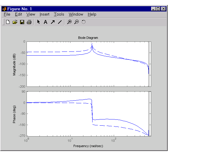
Now see how this compensator modifies the open-loop frequency response.

• bode(Hd,'--',oloop,'-')
  

The plant response is the dashed line and the open-loop response with the compensator is the solid line.

The plot above shows that the compensator has shifted up the phase plot (added lead) in the frequency range rad/sec.

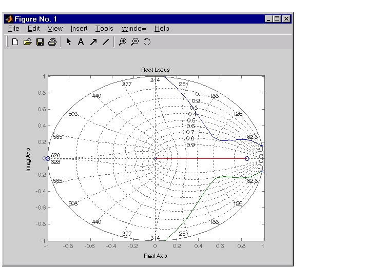
Now try the root locus again with the plant and compensator as open loop.

• rlocus(oloop)
  zgrid
  

Open the Property Editor by right-clicking in the plot away from the curve. On the Limits page, set the x- and y-axis limits from -1 to 1.01. This figure shows the result.

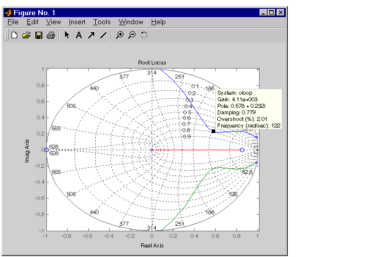
This time, the poles stay within the unit circle for some time (the lines drawn by zgrid show the damping ratios from to 1 in steps of 0.1). Use a data marker to find the point on the curve where the gain equals 4.111e+03. This figure shows the data marker at the correct location.

Adding a Compensator Gain

Design Analysis