kalman (Function Reference)

Design continuous- or discrete-time Kalman estimator

Syntax

[kest,L,P] = kalman(sys,Qn,Rn,Nn)
[kest,L,P,M,Z] = kalman(sys,Qn,Rn,Nn)   % discrete time only
[kest,L,P] = kalman(sys,Qn,Rn,Nn,sensors,known)

Description

kalman designs a Kalman state estimator given a state-space model of the plant and the process and measurement noise covariance data. The Kalman estimator is the optimal solution to the following continuous or discrete estimation problems.

Continuous-Time Estimation

Given the continuous plant

with known inputs and process and measurement white noise satisfying

construct a state estimate that minimizes the steady-state error covariance

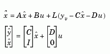
The optimal solution is the Kalman filter with equations

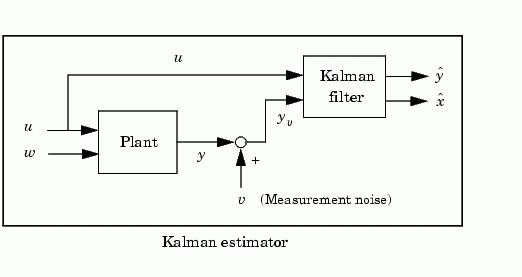
where the filter gain is determined by solving an algebraic Riccati equation. This estimator uses the known inputs and the measurements to generate the output and state estimates and . Note that estimates the true plant output

Discrete-Time Estimation

Given the discrete plant

and the noise covariance data

the Kalman estimator has equations

and generates optimal "current" output and state estimates and using all available measurements including . The gain matrices and are derived by solving a discrete Riccati equation. The innovation gain is used to update the prediction using the new measurement .

Usage

[kest,L,P] = kalman(sys,Qn,Rn,Nn) returns a state-space model kest of the Kalman estimator given the plant model sys and the noise covariance data Qn, Rn, Nn (matrices above). sys must be a state-space model with matrices

The resulting estimator kest has as inputs and (or their discrete-time counterparts) as outputs. You can omit the last input argument Nn when .

The function kalman handles both continuous and discrete problems and produces a continuous estimator when sys is continuous, and a discrete estimator otherwise. In continuous time, kalman also returns the Kalman gain L and the steady-state error covariance matrix P. Note that P is the solution of the associated Riccati equation. In discrete time, the syntax

```
[kest,L,P,M,Z] = kalman(sys,Qn,Rn,Nn)
```

returns the filter gain and innovations gain , as well as the steady-state error covariances

Finally, use the syntaxes

[kest,L,P] = kalman(sys,Qn,Rn,Nn,sensors,known)
[kest,L,P,M,Z] = kalman(sys,Qn,Rn,Nn,sensors,known)

for more general plants sys where the known inputs and stochastic inputs are mixed together, and not all outputs are measured. The index vectors sensors and known then specify which outputs of sys are measured and which inputs are known. All other inputs are assumed stochastic.

References

[1] Franklin, G.F., J.D. Powell, and M.L. Workman, Digital Control of Dynamic Systems, Second Edition, Addison-Wesley, 1990.