Getting Started

Creating Custom Plots

Time and frequency response commands are useful for creating custom plots. You can mix model response plots with other data views using response commands together with plot, subplot, and hold.

Example: Custom Plots

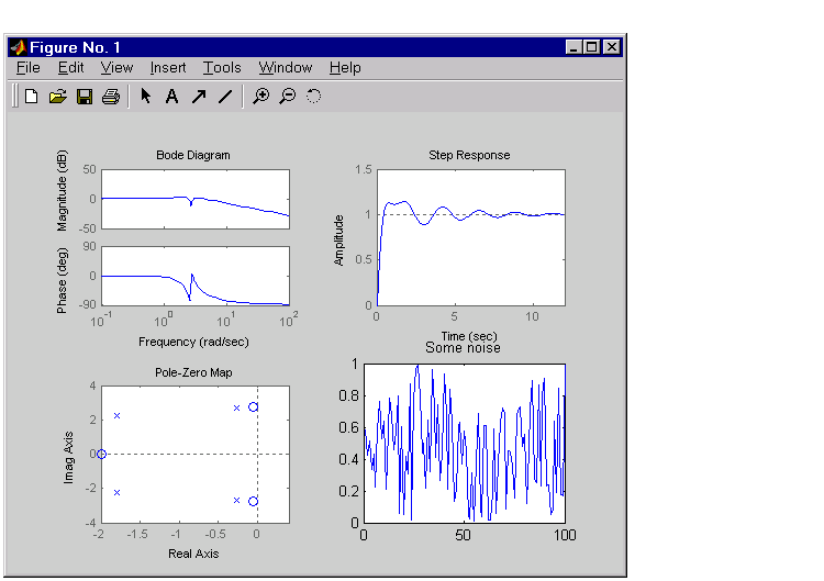
For example, the following sequence of commands displays the Bode plot, step response, pole/zero map, and some additional data in a single figure window.

• h = tf([4 8.4 30.8 60],[1 4.12 17.4 30.8 60]);
  subplot(221)
  bode(h)
  subplot(222)
  step(h)
  subplot(223)
  pzmap(h)
  subplot(224)
  plot(rand(1, 100))    % Any data can go here
  title('Some noise')
  

Your plot should look similar to this illustration.

Figure 3-18: Example of Model and Nonmodel Data Plotted in One Window

For information about plot, subplot, hold, and other options for plotting general data, see Basic Plots and Graphs in the MATLAB Function Reference. These documents are available in the MATLAB online help.

Note    Each of the plots generated by response analysis functions in Figure 3-18 (bode, step, and pzmap) has its own right-click menu (similar to those in the LTI Viewer). To activate the right-click menus, place your mouse in the plot region and right-click. The menu contents depend on what type of plot you have selected.

Plotting and Comparing Multiple Systems

Simulink LTI Viewer