Wavelet Toolbox

Filters Used to Calculate the DWT and IDWT

For an orthogonal wavelet, in the multiresolution framework (see [Dau92] in Using Wavelet Packets), we start with the scaling function and the wavelet function . One of the fundamental relations is the twin-scale relation (dilation equation or refinement equation):

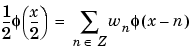
All the filters used in DWT and IDWT are intimately related to the sequence

Clearly if is compactly supported, the sequence (w_n) is finite and can be viewed as a filter. The filter W, which is called the scaling filter (nonnormalized), is

• Finite Impulse Response (FIR)
• Of length 2N
• Of sum 1
• Of norm
  
  
  
• A low-pass filter

For example, for the db3 scaling filter,

• load db3 
  db3
      db3 =
      0.2352   0.5706   0.3252  -0.0955  -0.0604   0.0249
  
  sum(db3)
      ans =
           1.0000
  
  norm(db3)
      ans =
           0.7071
  

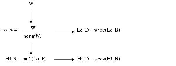
From filter W, we define four FIR filters, of length 2N and of norm 1, organized as follows.

Filters	Low-Pass	High-Pass
Decomposition	Lo_D	Hi_D
Reconstruction	Lo_R	Hi_R

The four filters are computed using the following scheme.

where qmf is such that Hi_R and Lo_R are quadrature mirror filters (i.e., Hi_R(k) = (-1) k Lo_R(2N + 1 - k)) for k = 1, 2, ..., 2N.

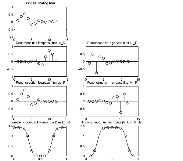
Note that wrev flips the filter coefficients. So Hi_D and Lo_D are also quadrature mirror filters. The computation of these filters is performed using orthfilt. Next, we illustrate these properties with the db6 wavelet. The plots associated with the following commands are shown in Figure 6-8,.

• % Load scaling filter.
  load db6; w = db6; 
  subplot(421); stem(w); title('Original scaling filter');
  
  % Compute the four filters.
  [Lo_D,Hi_D,Lo_R,Hi_R] = orthfilt(w); 
  subplot(423); stem(Lo_D); 
  title('Decomposition low-pass filter Lo{\_}D'); 
  subplot(424); stem(Hi_D); 
  title('Decomposition high-pass filter Hi{\_}D'); 
  subplot(425); stem(Lo_R); 
  title('Reconstruction low-pass filter Lo{\_}R'); 
  subplot(426); stem(Hi_R); 
  title('Reconstruction high-pass filter Hi{\_}R');
  
  % High and low frequency illustration.
  n = length(Hi_D);
  freqfft = (0:n-1)/n;
  nn = 1:n;
  N = 10*n;
  for k=1:N
      lambda(k) = (k-1)/N;
      XLo_D(k) = exp(-2*pi*j*lambda(k)*(nn-1))*Lo_D';
      XHi_D(k) = exp(-2*pi*j*lambda(k)*(nn-1))*Hi_D';
  end
  fftld = fft(Lo_D);
  ffthd = fft(Hi_D);
  subplot(427); plot(lambda,abs(XLo_D),freqfft,abs(fftld),'o'); 
  title('Transfer modulus: lowpass (Lo{\_}D or Lo{\_}R') 
  subplot(428); plot(lambda,abs(XHi_D),freqfft,abs(ffthd),'o'); 
  title('Transfer modulus: highpass (Hi{\_}D or Hi{\_}R') 
  
  
  

Figure 6-8: The Four Wavelet Filters for db6

The Fast Wavelet Transform (FWT) Algorithm

Algorithms