Statistics Toolbox

K-Means Clustering

This section gives a description and an example of using the MATLAB function for K-means clustering, kmeans.

• Overview of K-Means Clustering
• Example: Clustering Data in Four Dimensions

Overview of K-Means Clustering

K-means clustering can best be described as a partitioning method. That is, the function kmeans partitions the observations in your data into K mutually exclusive clusters, and returns a vector of indices indicating to which of the k clusters it has assigned each observation. Unlike the hierarchical clustering methods used in linkage (see Hierarchical Clustering), kmeans does not create a tree structure to describe the groupings in your data, but rather creates a single level of clusters. Another difference is that K-means clustering uses the actual observations of objects or individuals in your data, and not just their proximities. These differences often mean that kmeans is more suitable for clustering large amounts of data.

kmeans treats each observation in your data as an object having a location in space. It finds a partition in which objects within each cluster are as close to each other as possible, and as far from objects in other clusters as possible. You can choose from five different distance measures, depending on the kind of data you are clustering.

Each cluster in the partition is defined by its member objects and by its centroid, or center. The centroid for each cluster is the point to which the sum of distances from all objects in that cluster is minimized. kmeans computes cluster centroids differently for each distance measure, to minimize the sum with respect to the measure that you specify.

kmeans uses an iterative algorithm that minimizes the sum of distances from each object to its cluster centroid, over all clusters. This algorithm moves objects between clusters until the sum cannot be decreased further. The result is a set of clusters that are as compact and well-separated as possible. You can control the details of the minimization using several optional input parameters to kmeans, including ones for the initial values of the cluster centroids, and for the maximum number of iterations.

Example: Clustering Data in Four Dimensions

This example explores possible clustering in four-dimensional data by analyzing the results of partitioning the points into three, four, and five clusters.

Note    Because each part of this example generates random numbers sequentially, i.e., without setting a new seed, you must perform all steps in sequence to duplicate the results shown. If you perform the steps out of sequence, the answers will be essentially the same, but the intermediate results, number of iterations, or ordering of the silhouette plots may differ. See Random Numbers in Examples to set the correct seed.

Creating Clusters and Determining Separation.   First, load some data.

• load kmeansdata;
  size(X)
  
  ans =
     560     4
  

Even though these data are four-dimensional, and cannot be easily visualized, kmeans enables you to investigate if a group structure exists in them. Call kmeans with k, the desired number of clusters, equal to 3. For this example, specify the city block distance measure, and use the default starting method of initializing centroids from randomly selected data points.

• idx3 = kmeans(X,3,'distance','city');
  

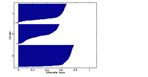
To get an idea of how well-separated the resulting clusters are, you can make a silhouette plot using the cluster indices output from kmeans. The silhouette plot displays a measure of how close each point in one cluster is to points in the neighboring clusters. This measure ranges from +1, indicating points that are very distant from neighboring clusters, through 0, indicating points that are not distinctly in one cluster or another, to -1, indicating points that are probably assigned to the wrong cluster. silhouette returns these values in its first output.

• [silh3,h] = silhouette(X,idx3,'city');
  xlabel('Silhouette Value')
  ylabel('Cluster')
  
  
  

From the silhouette plot, you can see that most points in the third cluster have a large silhouette value, greater than 0.6, indicating that that cluster is somewhat separated from neighboring clusters. However, the second cluster contains many points with low silhouette values, and the first contains a few points with negative values, indicating that those two clusters are not well separated.

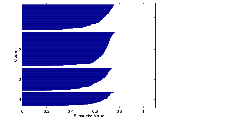
Determining the Correct Number of Clusters.   Increase the number of clusters to see if kmeans can find a better grouping of the data. This time, use the optional 'display' parameter to print information about each iteration.

• idx4 = kmeans(X,4, 'dist','city', 'display','iter');
    iter phase     num         sum
       1     1     560     2897.56
       2     1      53     2736.67
       3     1      50     2476.78
       4     1     102     1779.68
       5     1       5      1771.1
       6     2       0      1771.1
  6 iterations, total sum of distances = 1771.1
  

Notice that the total sum of distances decreases at each iteration as kmeans reassigns points between clusters and recomputes cluster centroids. In this case, the second phase of the algorithm did not make any reassignments, indicating that the first phase reached a minimum after five iterations. In some problems, the first phase may not reach a minimum, but the second phase always will.

A silhouette plot for this solution indicates that these four clusters are better separated than the three in the previous solution.

• [silh4,h] = silhouette(X,idx4,'city');
  xlabel('Silhouette Value')
  ylabel('Cluster')
  
  
  

A more quantitative way to compare the two solutions is to look at the average silhouette values for the two cases.

• mean(silh3)
  ans =
        0.52594
  
  mean(silh4)
  ans =
        0.63997
  

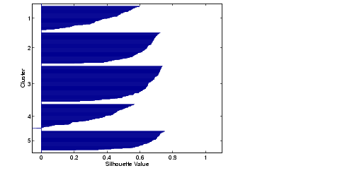
Finally, try clustering the data using five clusters.

• idx5 = kmeans(X,5,'dist','city','replicates',5);
  [silh5,h] = silhouette(X,idx5,'city');
  xlabel('Silhouette Value')
  ylabel('Cluster')
  mean(silh5)
  ans =
        0.52657
  
  
  

This silhouette plot indicates that this is probably not the right number of clusters, since two of the clusters contain points with mostly low slhouette values. Without some knowledge of how many clusters are really in the data, it is a good idea to experiment with a range of values for k.

Avoiding Local Minima.   Like many other types of numerical minimizations, the solution that kmeans reaches often depends on the starting points. It is possible for kmeans to reach a local minimum, where reassigning any one point to a new cluster would increase the total sum of point-to-centroid distances, but where a better solution does exist. However, you can use the optional 'replicates' parameter to overcome that problem.

For four clusters, specify five replicates, and use the 'display' parameter to print out the final sum of distances for each of the solutions.

• [idx4,cent4,sumdist] = kmeans(X,4,'dist','city',...
                         'display','final','replicates',5);
  17 iterations, total sum of distances = 2303.36
   5 iterations, total sum of distances = 1771.1
   6 iterations, total sum of distances = 1771.1
   5 iterations, total sum of distances = 1771.1
   8 iterations, total sum of distances = 2303.36
  

The output shows that, even for this relatively simple problem, non-global minima do exist. Each of these five replicates began from a different randomly selected set of initial centroids, and kmeans found two different local minima. However, the final solution that kmeans returns is the one with the lowest total sum of distances, over all replicates.

• sum(sumdist)
  ans =
         1771.1
  

Hierarchical Clustering

Classical Multidimensional Scaling