Welcome to Time Series Representation Methods and Similarity Measure Page

We welcome suggestions/bug fixes and donations of datasets/results.

This webpage provides supplementary materials to an experimental paper we submitted to VLDB conference 2008. Here you will find all the source code to our implementation, all the data sets we used in the experiments as well as additional experimental evaluation results.

DISCLAIMER: We have made the best effort to faithfully re-implement all the algorithms evaluated in this project, and compare them in the most possibly fair manner. The purpose of this project is to provide a consolidation of existing works on querying and mining time series, and to serve as a starting point for providing references and benchmarks for future research on time series. The algorithms are the intellectual property of the original authors.

 Download Sourcecode and data sets:

 Additional materials:

We claimed that the amortized time for constrained DTW gets better for large datasets. For large enough datasets, constrained DTW is about as fast as Euclidean distance. Lets test this. We searched increasingly large random walk datasets, of size [50, 100, 200, 400, 800, 1600, 3200, 6400, 12800, 25600] for the one nearest neighbor to a random query. Each time series was of length 128. (results are averaged over 100 queries) We tried every warping window size from 1 to 5. Recall that on most of the small datasets at the UCR archive, the best warping window size tends to be less than five, and experiments in this file show that the best warping window gets smaller as the data gets bigger. We measured the fraction of distance calculations that are pruned by a linear time lower bounding test (the LB_Keogh) which takes as long as Euclidean distance O(n). The results below show that, even for relatively small datasets with a few hundred items, at least 90% of the distance calculations are pruned, and we therefore only do the actual DTW less than 10% of the time. For large datasets, even with the most pessimistic warping window width, 98% of the DTW calculations are pruned.

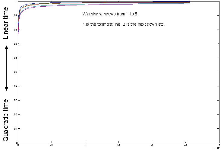
These results do not include other optimizations that you can do, finding a good match early on helps, because the best-so-far gets smaller more quickly and we can prune more. So indexing or hashing to an approximate match, then doing the scan helps. Also, the lower bound itself can use early abandoning [a].
Bottom Line: For sequential scanning, constrained DTW is about as fast as Euclidean distance for large datasets.

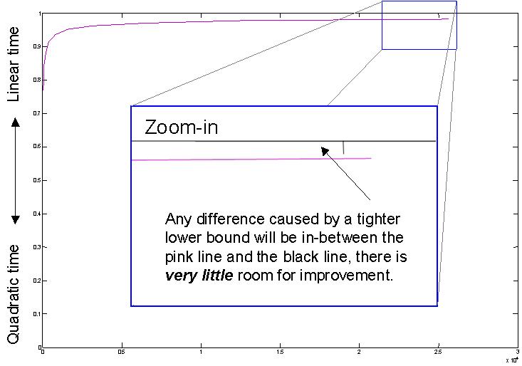
We can use the previous example to consider implications for tighter lower bounds. Occasionally there have been research efforts that attempt to create a tighter lower bound for DTW [b][c][d][e], could this help? Consider the figure below, which shows just the fraction of distance calculations pruned by LB_Keogh with a warping window of 5. Any improvement caused by a tighter lower bound will be in-between the pink line and the black line, there is very little room for improvement. In fact, some of the tighter lower bounds take more CPU time to compute, or they do not support early abandoning for the lower bound (see [a]) so they can be slower overall than the slightly weaker, but faster to compute lower bounds.

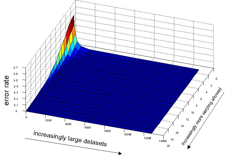
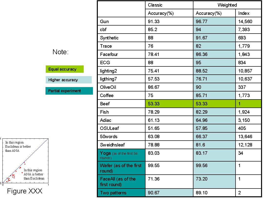
The next figure is an expanded version of a figure in our VLDB paper. We tested the error rate of nearest neighbor classification on the Two-Pattern dataset for the datasets sizes [50, 100, 200, 400, 800, 1600, 3,200, 6,400, 12,800] and over every DTW warping window width from 1 to 20. Recall that the case where DTW is 1 is the means it is the degenerate case of the Euclidean distance. What the figure shows is that if you have a small dataset, warping can help, and more warping is better up to some limit. However for larger datasets the effect diminishes. If you have a mere 2,000 objects, then Euclidean distance is as accurate at DTW. The take-home lessons are:

• If you have a lot of data , the accuracy of Euclidean distance may be very hard to beat.
• In spite of claims in the literature that say ¡°there may still be cases where unconstrained warping is useful¡± [a], this is not true here, and does not appear to be true on any of the 40 or so publicly available datasets with class labels. In other words, if you don¡¯t have a lot of data, just a little warping will be enough (thus allowing you to use lower bounds).

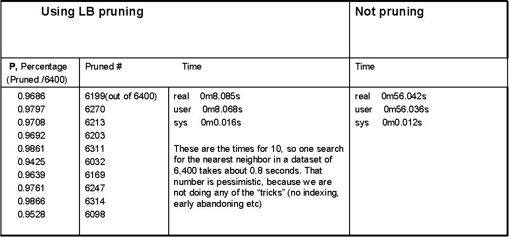
In the paper we note that the amortized cost of DTW on a large dataset is O((P * n) + (1-P nw)), where P is the fraction of the database pruned by a linear lower bound test. Below are the actual numbers for P on ten random queries. The queries where Two-Pat objects, but disjoint from the dataset searched (otherwise the results would be optimistic).

The next figure shows how we obtain the results for the Arbitrarily Naive Algorithm introduced in the appendix.

Finally, we show the full version of the three figures comparing the dimensionality reduction techniques in the paper.

First of all, the tightness of lower bounds for various time series representations on an ECG data set.

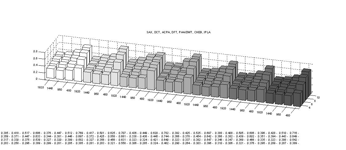
Next, the tightness of lower bounds for various time series representations on a relatively bursty data set

Third, The tightness of lower bounds for various time series representations on a periodic data set of tide levels

 Additional information on comparing similarity measures:

Table 1

Notes:

1. For an explaination on why we partition the data set into the number of crosses in the table, please refer to our paper.
2. DTW (w) means DTW with constrained warping window size, similarly, LCSS (w) means LCSS with constrained warping window size.
3. For the similarity measures that requires tuning, the results above are based on the parameters values that yield best performance with the tuning set. This is critical to avoid overfitting.
4. For an illustration on the data sets used in the experiments, click here.

Table 2

How to get the source code and the data sets: