Transforms (Image Processing Toolbox)

Image Processing Toolbox

The Inverse Radon Transform

The iradon function performs the inverse Radon transform, which is commonly used in tomography applications. This transform inverts the Radon transform (which was introduced in the previous section), and can therefore be used to reconstruct images from projection data.

As discussed in the previous section "Radon Transform" on page 8-21, given an image I and a set of angles theta, the function radon can be used to calculate the Radon transform.

```
R = radon(I,theta);
```

The function iradon can then be called to reconstruct the image I.

```
IR = iradon(R,theta);
```

In the example above, projections are calculated from the original image I. In most application areas, there is no original image from which projections are formed. For example, in X-ray absorption tomography, projections are formed by measuring the attenuation of radiation that passes through a physical specimen at different angles. The original image can be thought of as a cross section through the specimen, in which intensity values represent the density of the specimen. Projections are collected using special purpose hardware, and then an internal image of the specimen is reconstructed by iradon. This allows for noninvasive imaging of the inside of a living body or another opaque object.

iradon reconstructs an image from parallel beam projections. In parallel beam geometry, each projection is formed by combining a set of line integrals through an image at a specific angle.

Figure 8-17 below illustrates how parallel beam geometry is applied in X-ray absorption tomography. Note that there is an equal number of n emitters and n detectors. Each detector measures the radiation emitted from its corresponding emitter, and the attenuation in the radiation gives a measure of the integrated density, or mass, of the object. This corresponds to the line integral that is calculated in the Radon transform.

The parallel beam geometry used in the figure is the same as the geometry that was described under "Radon Transform" on page 8-21. f(x,y) denotes the brightness of the image and Rq(x´) is the projection at angle q.

Figure 8-17: Parallel Beam Projections Through an Object

Another geometry that is commonly used is fan beam geometry, in which there is one emitter and n detectors. There are methods for resorting sets of fan beam projections into parallel beam projections, which can then be used by iradon. (For more information on these methods, see Kak & Slaney, Principles of Computerized Tomographic Imaging, IEEE Press, NY, 1988, pp. 92-93.)

iradon uses the filtered backprojection algorithm to compute the inverse Radon transform. This algorithm forms an approximation to the image I based on the projections in the columns of R. A more accurate result can be obtained by using more projections in the reconstruction. As the number of projections (the length of theta) increases, the reconstructed image IR more accurately approximates the original image I. The vector theta must contain monotonically increasing angular values with a constant incremental angle . When the scalar is known, it can be passed to iradon instead of the array of theta values. Here is an example.

```
IR = iradon(R,Dtheta);
```

The filtered backprojection algorithm filters the projections in R and then reconstructs the image using the filtered projections. In some cases, noise can be present in the projections. To remove high frequency noise, apply a window to the filter to attenuate the noise. Many such windowed filters are available in iradon. The example call to iradon below applies a Hamming window to the filter. See the iradon reference page for more information.

```
IR = iradon(R,theta,'Hamming');
```

iradon also enables you to specify a normalized frequency, D, above which the filter has zero response. D must be a scalar in the range [0,1]. With this option, the frequency axis is rescaled, so that the whole filter is compressed to fit into the frequency range [0,D]. This can be useful in cases where the projections contain little high frequency information but there is high frequency noise. In this case, the noise can be completely suppressed without compromising the reconstruction. The following call to iradon sets a normalized frequency value of 0.85.

```
IR = iradon(R,theta,0.85);
```

Examples

The commands below illustrate how to use radon and iradon to form projections from a sample image and then reconstruct the image from the projections. The test image is the Shepp-Logan head phantom, which can be generated by the Image Processing Toolbox function phantom. The phantom image illustrates many of the qualities that are found in real-world tomographic imaging of human heads. The bright elliptical shell along the exterior is analogous to a skull, and the many ellipses inside are analogous to brain features or tumors.

```
P = phantom(256);
imshow(P)
```

As a first step the Radon transform of the phantom brain is calculated for three different sets of theta values. R1 has 18 projections, R2 has 36 projections, and R3 had 90 projections.

theta1 = 0:10:170; [R1,xp] = radon(P,theta1);
theta2 = 0:5:175;  [R2,xp] = radon(P,theta2);
theta3 = 0:2:178;  [R3,xp] = radon(P,theta3);

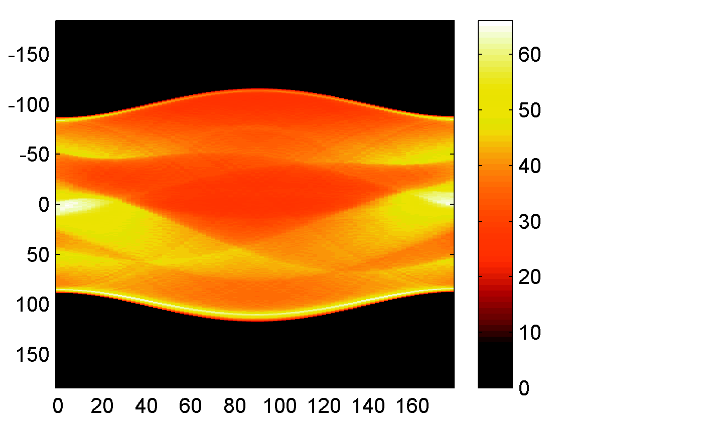
Now the Radon transform of the Shepp-Logan Head phantom is displayed using 90 projections (R3).

figure, imagesc(theta3,xp,R3); colormap(hot); colorbar
xlabel('\theta'); ylabel('x\prime');

Figure 8-18: Radon Transform of Head Phantom Using 90 Projections

When we look at Figure 8-18, we can see some of the features of the input image. The first column in the Radon transform corresponds to a projection at 0º which is integrating in the vertical direction. The centermost column corresponds to a projection at 90º, which is integrating in the horizontal direction. The projection at 90º has a wider profile than the projection at 0º due to the larger vertical semi-axis of the outermost ellipse of the phantom.

Figure 8-19 shows the inverse Radon transforms of R1, R2, and R3, which were generated above. Image I1 was reconstructed with the projections in R1, and it is the least accurate reconstruction, because it has the fewest projections. I2 was reconstructed with the 36 projections in R2, and the quality of the reconstruction is better, but it is still not clear enough to discern clearly the three small ellipses in the lower portion of the test image. I3 was reconstructed using the 90 projections in R3, and the result closely resembles the original image. Notice that when the number of projections is relatively small (as in I1 and I2), the reconstruction may include some artifacts from the back projection. To avoid this, use a larger number of angles.

I1 = iradon(R1,10);
I2 = iradon(R2,5);
I3 = iradon(R3,2);
imshow(I1)
figure, imshow(I2)
figure, imshow(I3)

Figure 8-19: Inverse Radon Transforms of the Shepp-Logan Head Phantom

Using the Radon Transform to Detect Lines Morphological Operations