Fixed-Point Blockset

1. Initial Guess at Scaling

In the first step, initial guesses for the scaling of each block are already specified in each block mask in the model. This step is included to illustrate the difficulty of guessing at the best scaling.

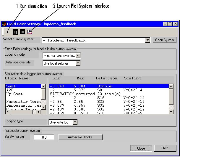
1. After you launch the Fixed-Point Settings interface, click the Run button in the dialog to run the simulation. When the simulation is finished, the Simulation data logged for current system pane of the interface displays the block name, the minimum and maximum simulation results, the data type, and the scaling for each block. The display shows that the Up Cast block saturated 23 times, indicating a poor guess for the scaling.
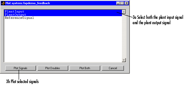
2. Click the Plot button. This launches the Plot System interface, which is shown below. This interface displays all MATLAB variable names that contain Scope block data for the current model.
3. To plot the simulation results, select one or more variable names in the Plot System interface, and then select the appropriate plot button. This simulation plots the fixed-point signals for the plant input and the plant output.

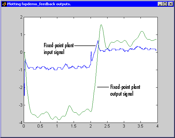
The plant input and output signals are shown below. These signals reflect the initial guess at scaling.

The Bode plot design sought to produce a well-behaved linear response for the closed-loop system. Clearly, the response is nonlinear. The nonlinear features are due to significant quantization effects. An important part of fixed-point design is finding scaling that reduce quantization effects to acceptable levels.

Simulation Results

2. Data Type Override