Getting Started

SISO Example: the DC Motor

A simple model of a DC motor driving an inertial load shows the angular rate of the load, , as the output and applied voltage, , as the input. The ultimate goal of this example is to control the angular rate by varying the applied voltage. This picture shows a simple model of the DC motor.

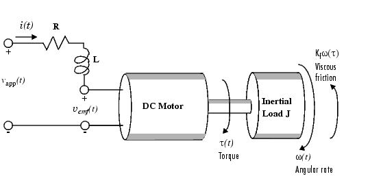
Figure 2-1: A Simple Model of a DC Motor Driving an Inertial Load

In this model, the dynamics of the motor itself are idealized; for instance, the magnetic field is assumed to be constant. The resistance of the circuit is denoted by R and the self-inductance of the armature by L. If you are unfamiliar with the basics of DC motor modeling, consult any basic text on physical modeling. The important thing here is that with this simple model and basic laws of physics, it is possible to develop differential equations that describe the behavior of this electromechanical system. In this example, the relationships between electric potential and mechanical force are Faraday's law of induction and Ampère's law for the force on a conductor moving through a magnetic field.

Mathematical Derivation

The torque seen at the shaft of the motor is proportional to the current i induced by the applied voltage,

where K_m, the armature constant, is related to physical properties of the motor, such as magnetic field strength, the number of turns of wire around the conductor coil, and so on. The back (induced) electromotive force, , is a voltage proportional to the angular rate seen at the shaft,

where K_b, the emf constant, also depends on certain physical properties of the motor.

The mechanical part of the motor equations is derived using Newton's law, which states that the inertial load J times the derivative of angular rate equals the sum of all the torques about the motor shaft. The result is this equation,

where is a linear approximation for viscous friction.

Finally, the electrical part of the motor equations can be described by

or, solving for the applied voltage and substituting for the back emf,

This sequence of equations leads to a set of two differential equations that describe the behavior of the motor, the first for the induced current,

and the second for the resulting angular rate.

State-Space Equations for the DC Motor

Given the two differential equations derived in the last section, you can now develop a state-space representation of the DC motor as a dynamical system. The current i and the angular rate are the two states of the system. The applied voltage, , is the input to the system, and the angular velocity is the output.

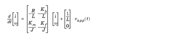
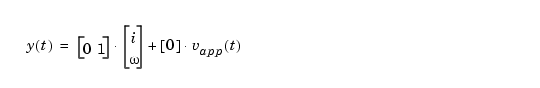
Figure 2-2: State-Space Representation of the DC Motor Example

Linear Model Representations

Constructing SISO Models