| Mathematics | |
MATLAB supports curve fitting through the Basic Fitting interface. Using this interface, you can quickly perform many curve fitting tasks within the same easy-to-use environment. The interface is designed so that you can:
Depending on your specific curve fitting application, you can use the Basic Fitting interface, the command line functionality, or both.
You can use the Basic Fitting interface only with 2-D data. However, if you plot multiple data sets as a subplot, and at least one data set is 2-D, then the interface is enabled.
| Note For the HP, IBM, and SGI platforms, the Basic Fitting interface is not supported for Release 13. |
Overview of the Basic Fitting Interface
The full Basic Fitting interface is shown below. To reproduce this state, follow these three steps:
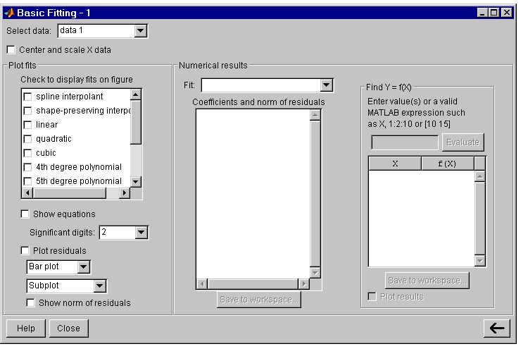
Select data - This parameter list is populated with the names of all the data sets you display in the figure window associated with the Basic Fitting interface.
Use this list to select the current data set. The current data set is defined as the data set that is to be fit. You can fit only one data set at a time. However, you can perform multiple fits for the current data set. Use the Plot Editor to change the name of a data set.
Center and scale X data - If checked, the data is centered at zero mean and scaled to unit standard deviation. You may need to center and scale your data to improve the accuracy of the subsequent numerical computations. A warning is displayed if a fit produces results that may be inaccurate.
Plot fits - This panel allows you to visually explore one or more fits to the current data set:
spline function, while the shape-preserving interpolant uses the pchip function. Refer to the pchip online help for a comparison of these two functions. The polynomial fits use the polyfit function. You can choose as many fits for a given data set as you want.
0 during the calculation so that the system is not underdetermined.
norm function, norm(V,2), where V is the vector of residuals.
Numerical results - This panel allows you to explore the numerical results of a single fit to the current data set without plotting the fit:
Example: Using the Basic Fitting Interface
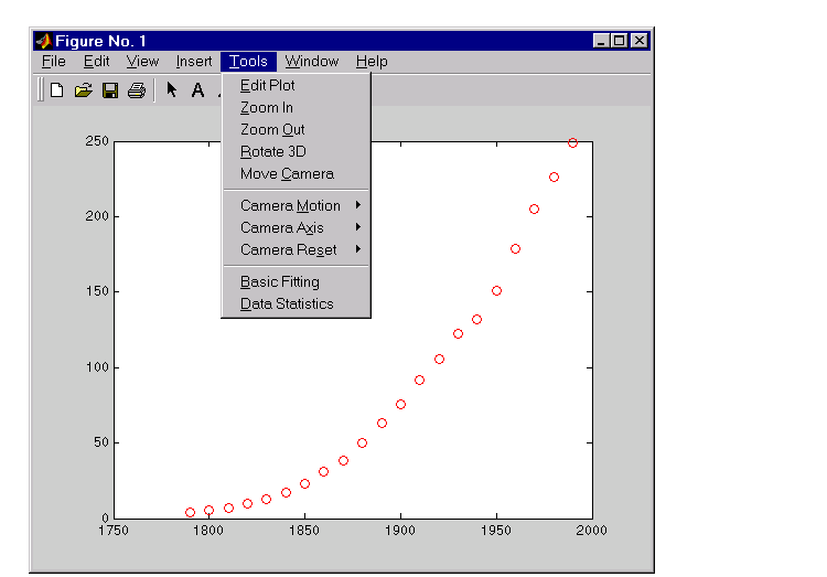
This example illustrates the features of the Basic Fitting interface by fitting a cubic polynomial to the census data. You may want to repeat this example using different equations and compare results. To launch the interface:
Configure the Basic Fitting interface to:
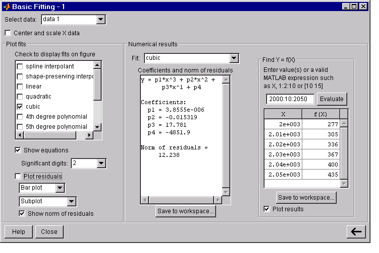
This configuration is shown below.
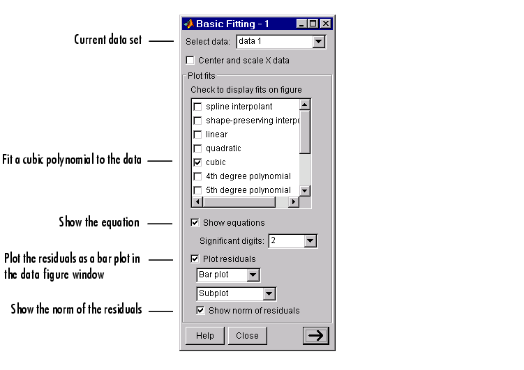
The Plot fits panel allows you to visually explore multiple fits to the current data set. For comparison, try fitting additional equations to the census data by selecting the appropriate check boxes. If an equation produces results that may be numerically inaccurate, a warning is displayed. In this case, you should select the Center and scale X data check box to improve the numerical accuracy.
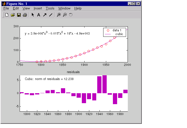
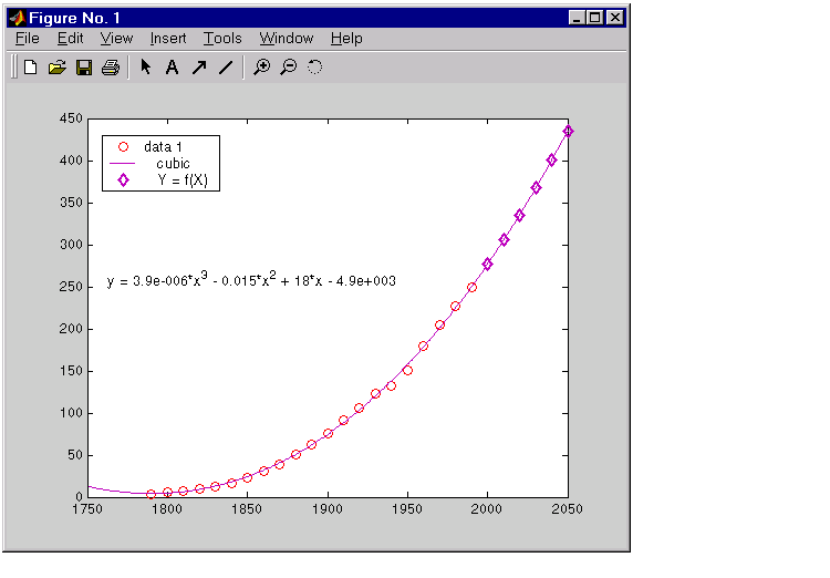
The resulting fit and the residuals are shown below.
The plot legend indicates the name of the data set and the equation. The legend is automatically updated as you add or remove data sets or fits. Additionally, fits are displayed using a default set of line styles and colors. You can change any of the default plot settings using the Plot Editor. However, any changes you make are undone if you subsequently perform another fit. To retain changes, you should wait until after you have finished fitting your data.
| Note If you change the name of a data set in the legend, then the name is automatically changed in the Select data menu. |
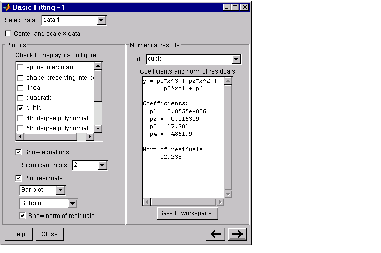
By selecting the  button, you can examine the fit coefficients and the norm of the residuals.
The Fit menu allows you to explore numerical fit results for the current data set without plotting the fit. For comparison, you can display the numerical results for other fits by selecting the desired equation. Note that if you want to display a fit in the data plot, you have to select the associated check box in Plot fits.
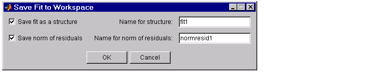
You can save the fit results to the MATLAB workspace by selecting the Save to workspace button.
The fit structure is shown below.
You may want to use this structure for subsequent display or analysis. For example, you can use the saved coefficients and the polyval function to evaluate the cubic polynomial at the command line.
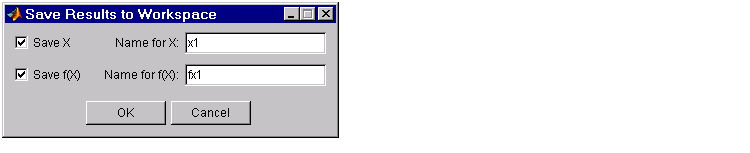
By selecting the button again, you can evaluate the current fit at the specified abscissa values. The current fit is displayed in the Fit menu. In this example, the population for the years 2000 to 2050 is evaluated in increments of 10, and then displayed in the data plot.
The evaluated data is shown below.
You can save the evaluated data to the MATLAB workspace by selecting the Save to workspace button.
| | Error Bounds | Difference Equations and Filtering | |