

| Writing S-Functions | |
Simple M-File S-Function Example
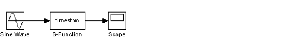
This block takes an input scalar signal, doubles it, and plots it to a scope.
The M-file code that contains the S-function is modeled on an S-function template called sfuntmpl.m, which is included with Simulink. By using this template, you can create an M-file S-function that is very close in appearance to a C MEX S-function. This is useful because it makes a transition from an M-file to a C MEX-file much easier.
Below is the M-file code for the timestwo.m S-function.
function [sys,x0,str,ts] = timestwo(t,x,u,flag)
% Dispatch the flag. The switch function controls the calls to
% S-function routines at each simulation stage.
switch flag,

   case 0
     [sys,x0,str,ts] = mdlInitializeSizes; % Initialization

   case 3
     sys = mdlOutputs(t,x,u); % Calculate outputs

   case { 1, 2, 4, 9 }
     sys = []; % Unused flags

   otherwise
     error(['Unhandled flag = ',num2str(flag)]); % Error handling
end;
% End of function timestwo.
Below are the S-function subroutines that timestwo.m calls.
%==============================================================
% Function mdlInitializeSizes initializes the states, sample
% times, state ordering strings (str), and sizes structure.
%==============================================================
function [sys,x0,str,ts] = mdlInitializeSizes
% Call function simsizes to create the sizes structure.
sizes = simsizes;
% Load the sizes structure with the initialization information.
sizes.NumContStates= 0;
sizes.NumDiscStates= 0;
sizes.NumOutputs=    1;
sizes.NumInputs=     1;
sizes.DirFeedthrough=1;
sizes.NumSampleTimes=1;
% Load the sys vector with the sizes information.
sys = simsizes(sizes);
%
x0 = []; % No continuous states
%
str = []; % No state ordering
%
ts = [-1 0]; % Inherited sample time
% End of mdlInitializeSizes.
%==============================================================
% Function mdlOutputs performs the calculations.
%==============================================================
function sys = mdlOutputs(t,x,u)
sys = 2*u;

% End of mdlOutputs.
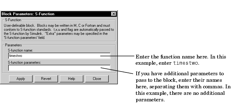
To test this S-function in Simulink, connect a sine wave generator to the input of an S-Function block. Connect the output of the S-Function block to a Scope. Double-click the S-Function block to open the dialog box.
You can now run this simulation.
Example - Continuous State S-Function
Simulink includes a function called csfunc.m, which is an example of a continuous state system modeled in an S-function. Here is the code for the M-file S-function.
function [sys,x0,str,ts] = csfunc(t,x,u,flag)
% CSFUNC An example M-file S-function for defining a system of
% continuous state equations:
%      x' = Ax + Bu
%      y  = Cx + Du
%
% Generate a continuous linear system:
A=[-0.09   -0.01
    1          0];
B=[ 1   -7
    0   -2];
C=[ 0    2
    1   -5];
D=[-3    0
    1    0];
%
% Dispatch the flag.
%
switch flag,

  case 0
    [sys,x0,str,ts]=mdlInitializeSizes(A,B,C,D); % Initialization

  case 1
    sys = mdlDerivatives(t,x,u,A,B,C,D); % Calculate derivatives

  case 3
    sys = mdlOutputs(t,x,u,A,B,C,D); % Calculate outputs

  case { 2, 4, 9 } % Unused flags
    sys = [];
  otherwise
    error(['Unhandled flag = ',num2str(flag)]); % Error handling
end
% End of csfunc.
%==============================================================
% mdlInitializeSizes
% Return the sizes, initial conditions, and sample times for the
% S-function.
%==============================================================
%
function [sys,x0,str,ts] = mdlInitializeSizes(A,B,C,D)
%
% Call simsizes for a sizes structure, fill it in and convert it
% to a sizes array.
%
sizes = simsizes;
sizes.NumContStates  = 2;
sizes.NumDiscStates  = 0;
sizes.NumOutputs     = 2;
sizes.NumInputs      = 2;
sizes.DirFeedthrough = 1;     % Matrix D is nonempty.
sizes.NumSampleTimes = 1;
sys = simsizes(sizes);
%
% Initialize the initial conditions.
%
x0 = zeros(2,1);
%
% str is an empty matrix.
%
str = [];
%
% Initialize the array of sample times; in this example the sample
% time is continuous, so set ts to 0 and its offset to 0.
%
ts = [0 0];
% End of mdlInitializeSizes.
%
%==============================================================
% mdlDerivatives
% Return the derivatives for the continuous states.
%==============================================================
function sys = mdlDerivatives(t,x,u,A,B,C,D)
sys = A*x + B*u;
% End of mdlDerivatives.
%
%==============================================================
% mdlOutputs
% Return the block outputs.
%==============================================================
%
function sys = mdlOutputs(t,x,u,A,B,C,D)
sys = C*x + D*u;
% End of mdlOutputs.
The preceding example conforms to the simulation stages discussed earlier in this chapter. Unlike timestwo.m, this example invokes mdlDerivatives to calculate the derivatives of the continuous state variables when flag = 1. The system state equations are of the form
so that very general sets of continuous differential equations can be modeled using csfunc.m. Note that csfunc.m is similar to the built-in State-Space block. This S-function can be used as a starting point for a block that models a state-space system with time-varying coefficients.
Each time the mdlDerivatives routine is called it must explicitly set the values of all derivatives. The derivative vector does not maintain the values from the last call to this routine. The memory allocated to the derivative vector changes during execution.
| | Examples of M-File S-Functions | Example - Discrete State S-Function | |