
| Signal Processing Toolbox |   |
Open the Filter Visualization Tool (FVTool)
Syntax
Description
fvtool(b,a)
opens FVTool and computes the magnitude response of the digital filter defined with numerator, b and denominator, a. Using FVTool you can display the phase response, group delay, impulse response, step response, pole-zero plot, and coefficients of the filter. You can export the displayed response to a file with Export on the File menu.
fvtool(b1,a1,b2,a2,...bn,an)
opens FVTool and computes the magnitude responses of multiple filters defined with numerators, b1...bn and denominators, a1...an.
fvtool(Hd1,Hd2,...)
opens FVTool and computes the magnitude responses of the filters in the dfilt objects Hd1, Hd2, etc. If you have the Filter Design Toolbox installed, you can also use fvtool on quantized filter (qfilt) objects by using fvtool(Hq1,Hq2,...).
h = fvtool(...)
returns the Handle Graphics figure handle h.
Linking to FDATool
In fdatool, selecting Full View Analysis from the Analysis menu or the Full View Analysis toolbar button
 launches FVTool for the current filter. You can synchronize FDATool and FVTool with the FDAToolLink toolbar button
  . Any changes made to the filter in FDATool are immediately reflected in FVTool.
Two FDAToolLink modes are provided via the Set Link Mode toolbar button :
 --removes the filter currently displayed in FVTool and inserts the new filter.
 --retains the filter currently displayed in FVTool and adds the new filter to the display.
Modifying the Axes
You can change the x- or y-axis units by right-clicking the mouse on the axis label or by right-clicking on the plot and selecting Analysis Parameters. Available options for the axes units are as follows.
Modifying the Plot
These toolbar buttons are provided for plot editing.
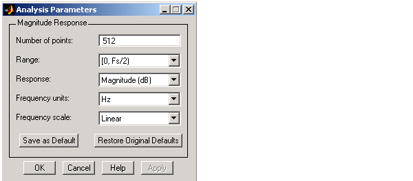
Analysis Parameters are parameters that apply to the displayed analysis. To display them, right-click in the plot area and select Analysis Parameters from the menu. (Note that you can access the menu only if the Edit Plot button is inactive.) The following analysis parameters are displayed. Not all of these analysis fields are displayed for all types of plots:
In addition to the above analysis parameters, you can change the plot type for Impulse and Step Response plots by right-clicking and selecting either Solid or Stem from the menu.
You can change the Sampling Frequency and names of your filters by right-clicking in the plot area and selecting Sampling Frequency from the menu. See Changing the Sampling Frequency for more information.
Data Markers display information about a particular point in the plot. See Using Data Markers for more information.
Example 1
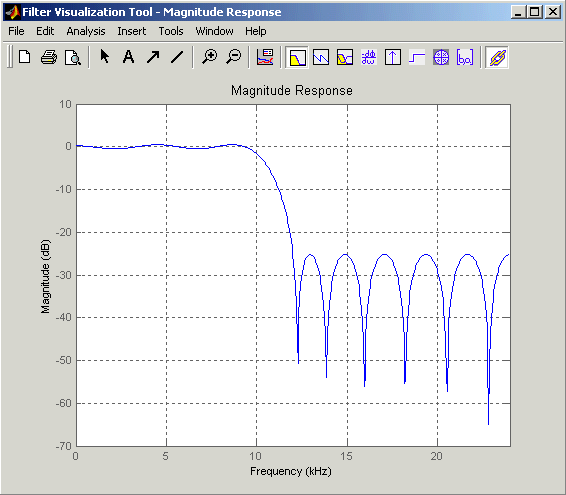
Display the magnitude response of an elliptic filter, starting FVTool from the command line:
Example 2
Display and analyze multiple FIR filters, starting FVTool from the command line. Then, display the associated analysis parameters for the magnitude:
n = 20;                  % Filter order
f = [0 0.4 0.5 1];       % Frequency band edges
a = [1 1 0 0];           % Desired amplitudes
b  = remez(n,f,a);
b2 = remez(n*2,f,a);     % Double the filter order
fvtool(b,1,b2,1);
Right-click on the plot and select Analysis Parameters.

Example 3
Create a lowpass, equiripple filter of order 20 in FDATool and display it in FVTool:
Set these parameters in fdatool and then click the Design Filter button.
Click the Full View Analysis button to launch FVTool.

See Also
 | freqz | gauspuls |  |