Design Case Studies

Time-Varying Design

Although the Control System Toolbox does not offer specific commands to perform time-varying Kalman filtering, it is easy to implement the filter recursions in MATLAB. This section shows how to do this for the stationary plant considered above.

First generate noisy output measurements

• % Use process noise w and measurement noise v generated above
  sys = ss(A,B,C,0,-1);
  y = lsim(sys,u+w);     % w = process noise
  yv = y + v;            % v = measurement noise
  

Given the initial conditions

you can implement the time-varying filter with the following for loop.

• P = B*Q*B';         % Initial error covariance
  x = zeros(3,1);     % Initial condition on the state
  ye = zeros(length(t),1);
  ycov = zeros(length(t),1); 
  
  for i=1:length(t)
    % Measurement update
    Mn = P*C'/(C*P*C'+R);
    x = x + Mn*(yv(i)-C*x);   % x[n|n]
    P = (eye(3)-Mn*C)*P;      % P[n|n]
  
    ye(i) = C*x;
    errcov(i) = C*P*C';
  
    % Time update
    x = A*x + B*u(i);        % x[n+1|n]
    P = A*P*A' + B*Q*B';     % P[n+1|n]
  end
  

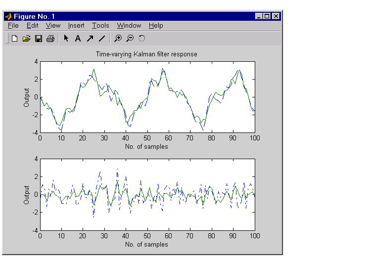
You can now compare the true and estimated output graphically.

• subplot(211), plot(t,y,'--',t,ye,'-')
  title('Time-varying Kalman filter response')
  xlabel('No. of samples'), ylabel('Output')
  subplot(212), plot(t,y-yv,'-.',t,y-ye,'-')
  xlabel('No. of samples'), ylabel('Output')
  
  
  
  

The first plot shows the true response (dashed line) and the filtered response (solid line). The second plot compares the measurement error (dash-dot) with the estimation error (solid).

The time-varying filter also estimates the covariance errcov of the estimation error at each sample. Plot it to see if your filter reached steady state (as you expect with stationary input noise).

• subplot(211)
  plot(t,errcov), ylabel('Error covar')
  
  
  
  

From this covariance plot, you can see that the output covariance did indeed reach a steady state in about five samples. From then on, your time-varying filter has the same performance as the steady-state version.

Compare with the estimation error covariance derived from the experimental data. Type

• EstErr = y-ye;
  EstErrCov = sum(EstErr.*EstErr)/length(EstErr)
  EstErrCov =
      0.2718
  

This value is smaller than the theoretical value errcov and close to the value obtained for the steady-state design.

Finally, note that the final value and the steady-state value of the innovation gain matrix coincide.

• Mn, M
  
  Mn =
      0.3798
      0.0817
     -0.2570
  
  M =
      0.3798
      0.0817
     -0.2570
  

Time-Varying Kalman Filter

References