Design Case Studies

Steady-State Design

You can design the steady-state Kalman filter described above with the function kalman. First specify the plant model with the process noise.

This is done by

• % Note: set sample time to -1 to mark model as discrete
  Plant = ss(A,[B B],C,0,-1,'inputname',{'u' 'w'},...
                            'outputname','y');
  

Assuming that , you can now design the discrete Kalman filter by

• Q = 1; R = 1;
  [kalmf,L,P,M] = kalman(Plant,Q,R);
  

This returns a state-space model kalmf of the filter as well as the innovation gain

• M
  
  M =
     3.7980e-01
     8.1732e-02
    -2.5704e-01
  

The inputs of kalmf are and , and its outputs are the plant output and state estimates and .

Because you are interested in the output estimate , keep only the first output of kalmf. Type

• kalmf = kalmf(1,:);
  kalmf
  a = 
                        x1_e         x2_e         x3_e
           x1_e       0.7683       -0.494       0.1129
           x2_e       0.6202            0            0
           x3_e    -0.081732            1            0
   
   
  b = 
                           u            y
           x1_e      -0.3832       0.3586
           x2_e       0.5919       0.3798
           x3_e       0.5191     0.081732
   
   
  c = 
                        x1_e         x2_e         x3_e
            y_e       0.6202            0            0
   
   
  d = 
                           u            y
            y_e            0       0.3798
   
  I/O groups:                            
        Group name      I/O    Channel(s)
        KnownInput       I         1     
       Measurement       I         2     
      OutputEstimate     O         1     
                                         
  Sampling time: unspecified
  Discrete-time model.
  

To see how the filter works, generate some input data and random noise and compare the filtered response with the true response . You can either generate each response separately, or generate both together. To simulate each response separately, use lsim with the plant alone first, and then with the plant and filter hooked up together. The joint simulation alternative is detailed next.

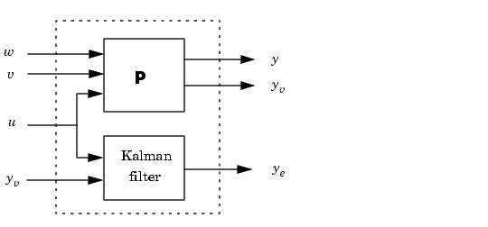
The block diagram below shows how to generate both true and filtered outputs.

You can construct a state-space model of this block diagram with the functions parallel and feedback. First build a complete plant model with as inputs and and (measurements) as outputs.

• a = A;
  b = [B B 0*B];
  c = [C;C];
  d = [0 0 0;0 0 1];
  P = ss(a,b,c,d,-1,'inputname',{'u' 'w' 'v'},...
                        'outputname',{'y' 'yv'});
  

Then use parallel to form the following parallel connection.

• sys = parallel(P,kalmf,1,1,[],[])
  

Finally, close the sensor loop by connecting the plant output to the filter input with positive feedback.

• % Close loop around input #4 and output #2
  SimModel = feedback(sys,1,4,2,1)
  % Delete yv from I/O list
  SimModel = SimModel([1 3],[1 2 3])
  

The resulting simulation model has as inputs and as outputs.

• SimModel.inputname
  
  ans = 
      'w'
      'v'
      'u'
  
  SimModel.outputname
  
  ans = 
      'y'
      'y_e'
  

You are now ready to simulate the filter behavior. Generate a sinusoidal input and process and measurement noise vectors and .

• t = [0:100]';
  u = sin(t/5);
  
  n = length(t)
  randn('seed',0)
  w = sqrt(Q)*randn(n,1);
  v = sqrt(R)*randn(n,1);
  

Now simulate with lsim.

• [out,x] = lsim(SimModel,[w,v,u]);
  
  y = out(:,1);   % true response
  ye = out(:,2);  % filtered response
  yv = y + v;     % measured response
  

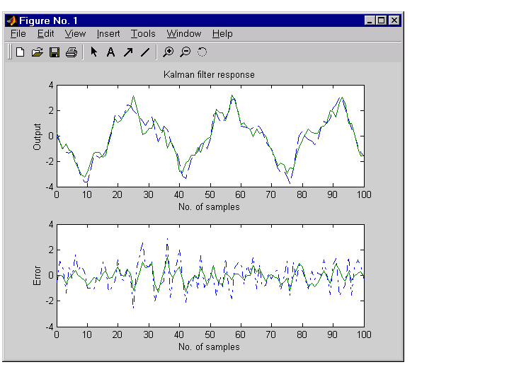
and compare the true and filtered responses graphically.

• subplot(211), plot(t,y,'--',t,ye,'-'), 
  xlabel('No. of samples'), ylabel('Output')
  title('Kalman filter response')
  subplot(212), plot(t,y-yv,'-.',t,y-ye,'-'),
  xlabel('No. of samples'), ylabel('Error')
  
  
  
  

The first plot shows the true response (dashed line) and the filtered output (solid line). The second plot compares the measurement error (dash-dot) with the estimation error (solid). This plot shows that the noise level has been significantly reduced. This is confirmed by the following error covariance computations.

• MeasErr = y-yv;
  MeasErrCov = sum(MeasErr.*MeasErr)/length(MeasErr);
  EstErr = y-ye;
  EstErrCov = sum(EstErr.*EstErr)/length(EstErr);
  

The error covariance before filtering (measurement error) is

• MeasErrCov
   
  MeasErrCov =
      1.1138
  

while the error covariance after filtering (estimation error) is only

• EstErrCov
   
  EstErrCov =
      0.2722
  

Discrete Kalman Filter

Time-Varying Kalman Filter