Design Case Studies

LQG Design for the x-Axis

As a first approximation, ignore the cross-coupling between the - and -axes and treat each axis independently. That is, design one SISO LQG regulator for each axis. The design objective is to reduce the thickness variations and due to eccentricity and input thickness disturbances.

Start with the -axis. First specify the model components as transfer function objects.

• % Hydraulic actuator (with input "u-x")
  Hx = tf(2.4e8,[1 72 90^2],'inputname','u-x')
  
  % Input thickness/hardness disturbance model
  Fix = tf(1e4,[1 0.05],'inputn','w-ix')
  
  % Rolling eccentricity model
  Fex = tf([3e4 0],[1 0.125 6^2],'inputn','w-ex')
  
  % Gain from force to thickness gap
  gx = 1e-6;
  

Next build the open-loop model shown in "Open-loop Model for x- or y-axis" above. You could use the function connect for this purpose, but it is easier to build this model by elementary append and series connections.

• % I/O map from inputs to forces f1 and f2
  Px = append([ss(Hx) Fex],Fix)
  
  % Add static gain from f1,f2 to outputs "x-gap" and "x-force" 
  Px = [-gx gx;1 1] * Px
  
  % Give names to the outputs:
  set(Px,'outputn',{'x-gap' 'x-force'})
  

Note    To obtain minimal state-space realizations, always convert transfer function models to state space before connecting them. Combining transfer functions and then converting to state space may produce nonminimal state-space models.

The variable Px now contains an open-loop state-space model complete with input and output names.

• Px.inputname
  
  ans = 
      'u-x'
      'w-ex'
      'w-ix'
  
  Px.outputname
  
  ans = 
      'x-gap'
      'x-force'
  

The second output 'x-force' is the rolling force measurement. The LQG regulator will use this measurement to drive the hydraulic actuator and reduce disturbance-induced thickness variations .

The LQG design involves two steps:

1. Design a full-state-feedback gain that minimizes an LQ performance measure of the form

2. Design a Kalman filter that estimates the state vector given the force measurements 'x-force'.

The performance criterion penalizes low and high frequencies equally. Because low-frequency variations are of primary concern, eliminate the high-frequency content of with the low-pass filter and use the filtered value in the LQ performance criterion.

• lpf = tf(30,[1 30])
  
  % Connect low-pass filter to first output of Px
  Pxdes = append(lpf,1) * Px
  set(Pxdes,'outputn',{'x-gap*' 'x-force'})
  
  % Design the state-feedback gain using LQRY and q=1, r=1e-4
  kx = lqry(Pxdes(1,1),1,1e-4)
  

Note    lqry expects all inputs to be commands and all outputs to be measurements. Here the command 'u-x' and the measurement 'x-gap*' (filtered gap) are the first input and first output of Pxdes. Hence, use the syntax Pxdes(1,1) to specify just the I/O relation between 'u-x' and 'x-gap*'.

Next, design the Kalman estimator with the function kalman. The process noise

has unit covariance by construction. Set the measurement noise covariance to 1000 to limit the high frequency gain, and keep only the measured output 'x-force' for estimator design.

• estx = kalman(Pxdes(2,:),eye(2),1000)
  

Finally, connect the state-feedback gain kx and state estimator estx to form the LQG regulator.

• Regx = lqgreg(estx,kx)
  

This completes the LQG design for the -axis.

Let's look at the regulator Bode response between 0.1 and 1000 rad/sec.

• bode(Regx,{0.1 1000})
  
  
  
  

The phase response has an interesting physical interpretation. First, consider an increase in input thickness. This low-frequency disturbance boosts both output thickness and rolling force. Because the regulator phase is approximately 0^o at low frequencies, the feedback loop then adequately reacts by increasing the hydraulic force to offset the thickness increase. Now consider the effect of eccentricity. Eccentricity causes fluctuations in the roll gap (gap between the rolling cylinders). When the roll gap is minimal, the rolling force increases and the beam thickness diminishes. The hydraulic force must then be reduced (negative force feedback) to restore the desired thickness. This is exactly what the LQG regulator does as its phase drops to -180^o near the natural frequency of the eccentricity disturbance (6 rad/sec).

Next, compare the open- and closed-loop responses from disturbance to thickness gap. Use feedback to close the loop. To help specify the feedback connection, look at the I/O names of the plant Px and regulator Regx.

• Px.inputname
  ans = 
      'u-x'
      'w-ex'
      'w-ix'
   
  Regx.outputname
  ans = 
      'u-x'
   
  Px.outputname
  ans = 
      'x-gap'
      'x-force'
   
  Regx.inputname
  ans = 
      'x-force'
  

This indicates that you must connect the first input and second output of Px to the regulator.

• clx = feedback(Px,Regx,1,2,+1)    % Note: +1 for positive feedback
  

You are now ready to compare the open- and closed-loop Bode responses from disturbance to thickness gap.

• bode(Px(1,2:3),'--',clx(1,2:3),'-',{0.1 100})
  
  
  
  

The dashed lines show the open-loop response. Note that the peak gain of the eccentricity-to-gap response and the low-frequency gain of the input-thickness-to-gap response have been reduced by about 20 dB.

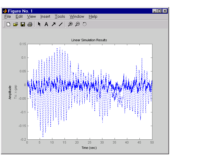
Finally, use lsim to simulate the open- and closed-loop time responses to the white noise inputs and . Choose dt=0.01 as sampling period for the simulation, and derive equivalent discrete white noise inputs for this sampling rate.

• dt = 0.01
  t = 0:dt:50   % time samples
  
  % Generate unit-covariance driving noise wx = [w-ex;w-ix].
  % Equivalent discrete covariance is 1/dt
  wx = sqrt(1/dt) * randn(2,length(t))
  
  lsim(Px(1,2:3),':',clx(1,2:3),'-',wx,t)
  
  
  
  

The dotted lines correspond to the open-loop response. In this simulation, the LQG regulation reduces the peak thickness variation by a factor 4.

Process and Disturbance Models

LQG Design for the y-Axis