| Wavelet Toolbox | |
Analysis of the Midday Period
This signal (see Example 14: A Real Electricity Consumption Signal) is also analyzed more crudely in Example 14: A Real Electricity Consumption Signal.
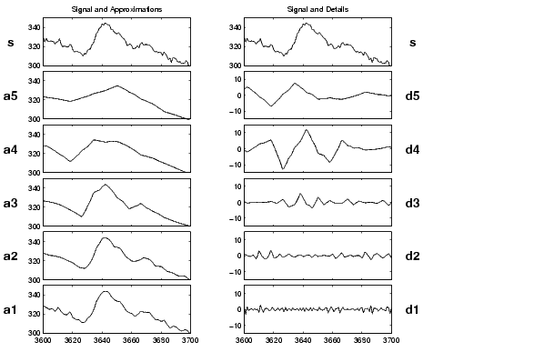
The shape is a middle mode between 12:30 p.m. and 1:00 p.m., preceded and followed by a hollow off-peak, and next a second smoother mode at 1:15 p.m. The approximation A5, corresponding to the time scale of 32 minutes, is a very crude approximation, particularly for the central mode: there is a peak time lag and an underestimation of the maximum value. So at this level, the most essential information is missing. We have to look at lower scales (4 for instance).
Let us examine the corresponding details.
The details D1 and D2 have small values and may be considered as local short-period discrepancies caused by the high-frequency components of sensor and state noises. In this bandpass, these noises are essentially due to measurement errors and fast variations of the signal induced by millions of state changes of personal electrical appliances.
The detail D3 exhibits high values at times corresponding to the start and the end of the original middle mode. It allows time localization of the local minima.
The detail D4 contains the main patterns: three successive modes. It is remarkably close to the shape of the curve. The ratio of the values of this level to the other levels is equal to 5. The detail D5 does not bear much information. So the contribution of the level 4 is the highest one, both in qualitative and quantitative aspects. It captures the shape of the curve in the concerned period.
In conclusion, with respect to the approximation A5, the detail D4 is the main additional correction: the components of a period of 8 to 16 minutes contain the crucial dynamics.
| | Data and the External Information | Analysis of the End of the Night Period | |