Writing S-Functions

Example of a Continuous State S-Function

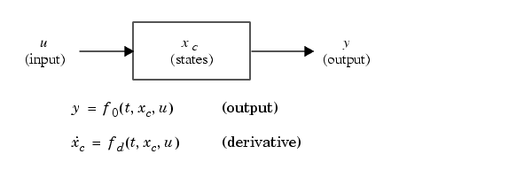
The matlabroot/simulink/src/csfunc.c example shows how to model a continuous system with states in a C MEX S-function. In continuous state integration, there is a set of states that Simulink's solvers integrate using the following equations.

S-functions that contain continuous states implement a state-space equation. The output portion is placed in mdlOutputs and the derivative portion in mdlDerivatives. To visualize how the integration works, refer to the flowchart in How Simulink Interacts with C S-Functions. The output equation above corresponds to the mdlOutputs in the major time step. Next, the example enters the integration section of the flowchart. Here Simulink performs a number of minor time steps during which it calls mdlOutputs and mdlDerivatives. Each of these pairs of calls is referred to as an integration stage. The integration returns with the continuous states updated and the simulation time moved forward. Time is moved forward as far as possible, providing that error tolerances in the state are met. The maximum time step is subject to constraints of discrete events such as the actual simulation stop time and the user-imposed limit.

Note that csfunc.c specifies that the input port has direct feedthrough. This is because matrix D is initialized to a nonzero matrix. If D is set equal to a zero matrix in the state-space representation, the input signal isn't used in mdlOutputs. In this case, the direct feedthrough can be set to 0, which indicates that csfunc.c does not require the input signal when executing mdlOutputs.

matlabroot/simulink/src/csfunc.c

• /*  File    : csfunc.c
   *  Abstract:
   *
   *      Example C-file S-function for defining a continuous system.  
   *
   *      x' = Ax + Bu
   *      y  = Cx + Du
   *
   *      For more details about S-functions, see simulink/src/sfuntmpl_doc.c.
   * 
   *  Copyright 1990-2000 The MathWorks, Inc.
   */
  
  #define S_FUNCTION_NAME csfunc
  #define S_FUNCTION_LEVEL 2
  
  #include "simstruc.h"
  
  #define U(element) (*uPtrs[element])  /* Pointer to Input Port0 */
  
  static real_T A[2][2]={ { -0.09, -0.01 } ,
                          {  1   ,  0    } 
                        };
  
  static real_T B[2][2]={ {  1   , -7    } ,
                          {  0   , -2    } 
                        };
  
  static real_T C[2][2]={ {  0   , 2     } ,
                          {  1   , -5    } 
                        };
  
  static real_T D[2][2]={ { -3   , 0     } ,
                          {  1   , 0     } 
                        };
  
  /*====================*
   * S-function methods *
   *====================*/
  
  /* Function: mdlInitializeSizes ===============================================
   * Abstract:
   *    The sizes information is used by Simulink to determine the S-function
   *    block's characteristics (number of inputs, outputs, states, etc.).
   */
  static void mdlInitializeSizes(SimStruct *S)
  {
      ssSetNumSFcnParams(S, 0);  /* Number of expected parameters */
      if (ssGetNumSFcnParams(S) != ssGetSFcnParamsCount(S)) {
          return; /* Parameter mismatch will be reported by Simulink */
      }
  
      ssSetNumContStates(S, 2);
      ssSetNumDiscStates(S, 0);
  
      if (!ssSetNumInputPorts(S, 1)) return;
      ssSetInputPortWidth(S, 0, 2);
      ssSetInputPortDirectFeedThrough(S, 0, 1);
  
      if (!ssSetNumOutputPorts(S, 1)) return;
      ssSetOutputPortWidth(S, 0, 2);
  
      ssSetNumSampleTimes(S, 1);
      ssSetNumRWork(S, 0);
      ssSetNumIWork(S, 0);
      ssSetNumPWork(S, 0);
      ssSetNumModes(S, 0);
      ssSetNumNonsampledZCs(S, 0);
  
      /* Take care when specifying exception free code - see sfuntmpl_doc.c */
      ssSetOptions(S, SS_OPTION_EXCEPTION_FREE_CODE);
  }
  
  
  
  /* Function: mdlInitializeSampleTimes =========================================
   * Abstract:
   *    Specifiy that we have a continuous sample time.
   */
  static void mdlInitializeSampleTimes(SimStruct *S)
  {
      ssSetSampleTime(S, 0, CONTINUOUS_SAMPLE_TIME);
      ssSetOffsetTime(S, 0, 0.0);
  }
  
  
  
  #define MDL_INITIALIZE_CONDITIONS
  /* Function: mdlInitializeConditions ========================================
   * Abstract:
   *    Initialize both continuous states to zero.
   */
  static void mdlInitializeConditions(SimStruct *S)
  {
      real_T *x0 = ssGetContStates(S);
      int_T  lp;
  
      for (lp=0;lp<2;lp++) { 
          *x0++=0.0; 
      }
  }
  
  
  
  /* Function: mdlOutputs =======================================================
   * Abstract:
   *      y = Cx + Du 
   */
  static void mdlOutputs(SimStruct *S, int_T tid)
  {
      real_T            *y    = ssGetOutputPortRealSignal(S,0);
      real_T            *x    = ssGetContStates(S);
      InputRealPtrsType uPtrs = ssGetInputPortRealSignalPtrs(S,0);
   
      UNUSED_ARG(tid); /* not used in single tasking mode */
  
      /* y=Cx+Du */
      y[0]=C[0][0]*x[0]+C[0][1]*x[1]+D[0][0]*U(0)+D[0][1]*U(1);
      y[1]=C[1][0]*x[0]+C[1][1]*x[1]+D[1][0]*U(0)+D[1][1]*U(1);
  }
  
  
  
  #define MDL_DERIVATIVES
  /* Function: mdlDerivatives =================================================
   * Abstract:
   *      xdot = Ax + Bu
   */
  static void mdlDerivatives(SimStruct *S)
  {
      real_T            *dx   = ssGetdX(S);
      real_T            *x    = ssGetContStates(S);
      InputRealPtrsType uPtrs = ssGetInputPortRealSignalPtrs(S,0);
  
      /* xdot=Ax+Bu */
      dx[0]=A[0][0]*x[0]+A[0][1]*x[1]+B[0][0]*U(0)+B[0][1]*U(1);
      dx[1]=A[1][0]*x[0]+A[1][1]*x[1]+B[1][0]*U(0)+B[1][1]*U(1);
  }
  
  /* Function: mdlTerminate =====================================================
   * Abstract:
   *    No termination needed, but we are required to have this routine.
   */
  static void mdlTerminate(SimStruct *S)
  {
      UNUSED_ARG(S); /* unused input argument */
  }
  
  #ifdef  MATLAB_MEX_FILE    /* Is this file being compiled as a MEX-file? */
  #include "simulink.c"      /* MEX-file interface mechanism */
  #else
  #include "cg_sfun.h"       /* Code generation registration function */
  #endif
  

S-Function Examples

Example of a Discrete State S-Function