
| Function Reference |   |
Singular values of the frequency response of LTI models
Syntax
sigma(sys)
sigma(sys,w)
sigma(sys,w,type)

sigma(sys1,sys2,...,sysN)
sigma(sys1,sys2,...,sysN,w)
sigma(sys1,sys2,...,sysN,w,type)
sigma(sys1,'PlotStyle1',...,sysN,'PlotStyleN')

[sv,w] = sigma(sys)
sv = sigma(sys,w)
Description
sigma
calculates the singular values of the frequency response of an LTI model. For an FRD model, sys, sigma computes the singular values of sys.Response at the frequencies, sys.frequency. For continuous-time TF, SS, or ZPK models with transfer function  ,
, sigma computes the singular values of  as a function of the frequency
  . For discrete-time TF, SS, or ZPK models with transfer function
  and sample time
  ,
, sigma computes the singular values of

for frequencies  between 0 and the Nyquist frequency
  .
.
The singular values of the frequency response extend the Bode magnitude response for MIMO systems and are useful in robustness analysis. The singular value response of a SISO system is identical to its Bode magnitude response. When invoked without output arguments, sigma produces a singular value plot on the screen.
sigma(sys)
plots the singular values of the frequency response of an arbitrary LTI model sys. This model can be continuous or discrete, and SISO or MIMO. The frequency points are chosen automatically based on the system poles and zeros, or from sys.frequency if sys is an FRD.
sigma(sys,w)
explicitly specifies the frequency range or frequency points to be used for the plot. To focus on a particular frequency interval [wmin,wmax], set w = {wmin,wmax}. To use particular frequency points, set w to the corresponding vector of frequencies. Use logspace to generate logarithmically spaced frequency vectors. The frequencies must be specified in rad/sec.
sigma(sys,[],type) or sigma(sys,w,type) plots the following modified singular value responses:
|
Singular values of the frequency response |
|
|
|
Singular values of the frequency response  . . |
These options are available only for square systems, that is, with the same number of inputs and outputs.
To superimpose the singular value plots of several LTI models on a single figure, use
sigma(sys1,sys2,...,sysN)sigma(sys1,sys2,...,sysN,[],type) % modified SV plotsigma(sys1,sys2,...,sysN,w) % specify frequency range/grid
The models sys1,sys2,...,sysN need not have the same number of inputs and outputs. Each model can be either continuous- or discrete-time. You can also specify a distinctive color, linestyle, and/or marker for each system plot with the syntax
When invoked with output arguments,
return the singular values sv of the frequency response at the frequencies w. For a system with Nu input and Ny outputs, the array sv has min(Nu,Ny) rows and as many columns as frequency points (length of w). The singular values at the frequency w(k) are given by sv(:,k).
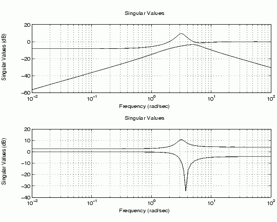
Example
Plot the singular value responses of

H = [0 tf([3 0],[1 1 10]) ; tf([1 1],[1 5]) tf(2,[1 6])]

subplot(211)
sigma(H)
subplot(212)
sigma(H,[],2)
Algorithm
sigma uses the svd function in MATLAB to compute the singular values of a complex matrix.
See Also
bode Bode plot
evalfr Response at single complex frequency
freqresp Frequency response computation
ltiview LTI system viewer
nichols Nichols plot
nyquist Nyquist plot
 | sgrid | sisotool |  |