Tutorial (System Identification Toolbox)

System Identification Toolbox

Structured State-Space Models with Free Parameters: the idss Model

The System Identification Toolbox allows you to define arbitrary parameterizations of the matrices in (3-51) or (3-52). To define the structure, so called structure matrices are used. These are "shadow matrices" to A, B, C, D, K, and X0, and have the same sizes and coincide with these at all matrix elements that are known. The structure matrices are denoted by As, Bs, Cs, Ds, Ks, and X0s and have the entry NaN at those elements that correspond to unknown parameters to be estimated.

For example,

```
m.As = [NaN 0;0 NaN]
```

sets the structure matrix for A, called As, to a diagonal matrix, where the diagonal elements are freely adjustable. Defining

```
m.A = [2 0; 0 3]
```

sets the nominal/initial values of these diagonal elements to 2 and 3, respectively.

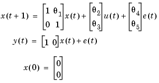
Example 3.1: A Discrete-Time Structure. Consider the discrete-time model

with five unknown parameters , i=1,...,5. Suppose the nominal/initial values of these parameters are -1, 2, 3, 4 and 5. This structure is then defined by

m = idss([1, -1;0, 1],[2;3],[1,0],0,[4;5])
m.As = [1, NaN; 0 ,1];
m.Bs = [NaN;NaN];
m.Cs = [1, 0];
m.Ds = 0;
m.Ks = [NaN;NaN];
m.x0s = [0;0];

The definition thus follows in two steps. First the nominal model is defined. Then the structure (known and unknown parameter values) is defined by the structure matrices, As, Bs, etc.

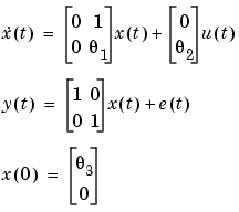
Example 3.2: A Continuous-Time Model Structure. Consider the following model structure

This corresponds to an electrical motor, where is the angular position of the motor shaft and is the angular velocity. The parameter is the inverse time constant of the motor and is the static gain from the input to the angular velocity. (See page Example 4.1 in Ljung (1999).) The motor is at rest at time 0 but at an unknown angular position. Suppose that is around -1 and is around 0.25. If you also know that the variance of the errors in the position measurement is 0.01 and in the angular velocity measurements is 0.1, you can then define an idss model using

m = idss([0 1;0 
    -1],[0;0.25],eye(2),[0;0],zeros(2,2),[0;0],'Ts',0)
m.as = [0 1; 0 NaN]
m.bs = [0 ;NaN]
m.cs = m.c
m.ds = m.d
m.ks = m.k
m.x0s = [NaN;0]
m.noisevar = [0.01 0; 0 0.1]

The structure m can now be used to estimate the unknown parameters from observed data

```
Data = iddata([y1 y2], u, 0.1)
```

```
model = pem(Data,m)
```

The iterative search for minimum is then initialized at the parameters in the nominal model m. The continuous time model is automatically sampled to agree with the sampling interval of the data. The structure can also be used to simulate the system above with sampling interval T=0.1 for input u and noise realization e.

e = randn(300,2)
u = idinput(300);
simdat = iddata([],[u e],'Ts',0.1);
y = sim(m,simdat) % The continuous system will automatically be 
                  % sampled using Ts =0.1

The nominal parameter values are then used, and the noise sequence is scaled according to the matrix m.noisevar.

When estimating models, you can try a number of "neighboring" structures, such as "what happens if I fix this parameter to a certain value" or "what happens if I let loose these parameters." This is easily handled by the structure matrices As, Bs, etc. For example, to free the parameter x₂(0) (perhaps the motor wasn't at rest after all), you can use

```
model = pem(Data,m,'x0s',[NaN;NaN])
```

To manipulate initial conditions, the function init is also useful.

Black-Box State-Space Models: the idss Model State-Space Models with Coupled Parameters: the idgrey Model