Overview (Financial Toolbox)

Financial Toolbox

Multiplying Matrices

Matrix multiplication does not operate element-by-element. It operates according to the rules of linear algebra. In multiplying matrices, it helps to remember this key rule: the inner dimensions must be the same. That is, if the first matrix is m-by-3, the second must be 3-by-n. The resulting matrix is m-by-n. It also helps to "talk through" the units of each matrix, as mentioned above.

Matrix multiplication also is not commutative; i.e., it is not independent of order. A*B does not equal B*A. The dimension rule illustrates this property. If A is 1-by-3 and B is 3-by-1, A*B yields a scalar (1-by-1) but B*A yields a 3-by-3 matrix.

Multiplying Vectors

Vector multiplication follows the same rules and helps illustrate the principles. For example, a stock portfolio has three different stocks and their closing prices today are

```
ClosePrices = [42.5   15   78.875]
```

The portfolio contains these numbers of shares of each stock.

NumShares = [100
             500
             300]

To find the value of the portfolio, simply multiply the vectors

```
PortfValue = ClosePrices * NumShares
```

which yields

PortfValue =

            35412.50

The vectors are 1-by-3 and 3-by-1; the resulting vector is 1-by-1, a scalar. Multiplying these vectors thus means multiplying each closing price by its respective number of shares and summing the result.

To illustrate order dependence, switch the order of the vectors

Values = NumShares * ClosePrices

Values =

       4250.00       1500.00       7887.50
      21250.00       7500.00      39437.50
      12750.00       4500.00      23662.50

which shows the closing values of 100, 500, and 300 shares of each stock -- not the portfolio value, and meaningless for this example.

Computing Dot Products of Vectors

In matrix algebra, if X and Y are vectors of the same length

then the dot product

is the scalar product of the two vectors. It is an exception to the commutative rule. To compute the dot product in MATLAB, use sum(X .* Y) or sum(Y .* X). Just be sure the two vectors have the same dimensions. To illustrate, use the previous vectors.

Value = sum(NumShares .* ClosePrices')

Value =

      35412.50

Value = sum(ClosePrices .* NumShares')

Value =

      35412.50

As expected, the value in these cases is exactly the same as the PortfValue computed previously.

Multiplying Vectors and Matrices

Multiplying vectors and matrices follows the matrix multiplication rules and process. For example, a portfolio matrix contains closing prices for a week. A second matrix (vector) contains the stock quantities in the portfolio.

WeekClosePr = [42.5     15      78.875
               42.125   15.5    78.75
               42.125   15.125  79
               42.625   15.25   78.875
               43       15.25   78.625];
PortQuan = [100
            500
            300];

To see the closing portfolio value for each day, simply multiply

WeekPortValue = WeekClosePr * PortQuan

WeekPortValue =

      35412.50
      35587.50
      35475.00
      35550.00
      35512.50

The prices matrix is 5-by-3, the quantity matrix (vector) is 3-by-1, so the resulting matrix (vector) is 5-by-1.

Multiplying Two Matrices

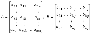
Matrix multiplication also follows the rules of matrix algebra. In matrix algebra notation, if A is an m-by-n matrix and B is an n-by-p matrix

then C = A*B is an m-by-p matrix; and the element c_ij in the ith row and jth column of C is

To illustrate, assume there are two portfolios of the same three stocks above but with different quantities.

Portfolios = [100   200
              500   400
              300   150];

Multiplying the 5-by-3 week's closing prices matrix by the 3-by-2 portfolios matrix yields a 5-by-2 matrix showing each day's closing value for both portfolios.

PortfolioValues = WeekClosePr * Portfolios

PortfolioValues =

      35412.50      26331.25
      35587.50      26437.50
      35475.00      26325.00
      35550.00      26456.25
      35512.50      26493.75

Monday's values result from multiplying each Monday closing price by its respective number of shares and summing the result for the first portfolio, then doing the same for the second portfolio. Tuesday's values result from multiplying each Tuesday closing price by its respective number of shares and summing the result for the first portfolio, then doing the same for the second portfolio. And so on through the rest of the week. With one simple command, MATLAB quickly performs many calculations.

Multiplying a Matrix by a Scalar

Multiplying a matrix by a scalar is an exception to the dimension and commutative rules. It just operates element-by-element.

Portfolios = [100   200
              500   400
              300   150];

DoublePort = Portfolios * 2

DoublePort =
        200.00        400.00
       1000.00        800.00
        600.00        300.00

Adding and Subtracting Matrices Dividing Matrices